Introduction
The full capabilities of CytoExploreR will be documented in series of vignettes which address specific aspects of the data analysis pipeline. Before we dive into the details, let’s walk through the basic steps to analyse some in vitro T cell activation data using CytoExploreR.
This Activation dataset and associated Compensation controls have been shipped with CytoExploreRData for demonstration purposes. This in vitro assay involves stimulating dendritic cells (DCs) with different immune stimulators (referred to as Stim-A, Stim-B, Stim-C and Stim-D) under increasing concentrations of the surrogate antigen ovalbumin (0 nM, 5 nM, 50 nM or 500 nM OVA). These activated DCs are then co-cultured with antigen-specific OT-I (CD8+) and OT-II (CD4+) T cells. The ability of each of the immune stimulators to promote T cell activation was then assessed by measuring the expression of T cell activation markers (CD44 and CD69) by flow cytometry.
Although CytoExploreR has full support for automated gating through openCyto, for simplicity in this vignette we will describe a manual gating analysis pipeline to analyse this dataset.1. Set Up New R Project
Before we begin, we will need to create a new R project by following these steps:
- Select File -> New Project
- Select New Directory -> New Project
- Set Directory Name to “CytoExploreR-Demo”
- Indicate where the project should be created and select Create Project
2. Load Required Packages
# Load required packages
library(CytoExploreR)
library(CytoExploreRData)
3. Save FCS Files
# Compensation FCS Files
cyto_save(Compensation,
          save_as = "Compensation-Samples")

# Activation FCS Files
cyto_save(Activation,
          save_as = "Activation-Samples")
4. Compensation of Fluorescent Spillover
4.1 Prepare compensation controls
cyto_setup. At this stage it is also a good idea to setup a new gatingTemplate to record any downstream gating operations. Once the compensation controls have been loaded into a GatingSet, we need to transform the fluorescent channels using cyto_transform. The transformed data can then be gated using cyto_gate_draw to remove debris and doublets to ensure accurate computation of spillover values.
# Setup compensation controls
gs <- cyto_setup("Compensation-Samples",
                 gatingTemplate = "Compensation-gatingTemplate.csv")

# Transform fluorescent channels - default logicle transformations
gs <- cyto_transform(gs)

# Gate Cells
cyto_gate_draw(gs,
               parent = "root",
               alias = "Cells",
               channels = c("FSC-A", "SSC-A"))

# Gate Single Cells
cyto_gate_draw(gs,
               parent = "Cells",
               alias = "Single Cells",
               channels = c("FSC-A", "FSC-H"))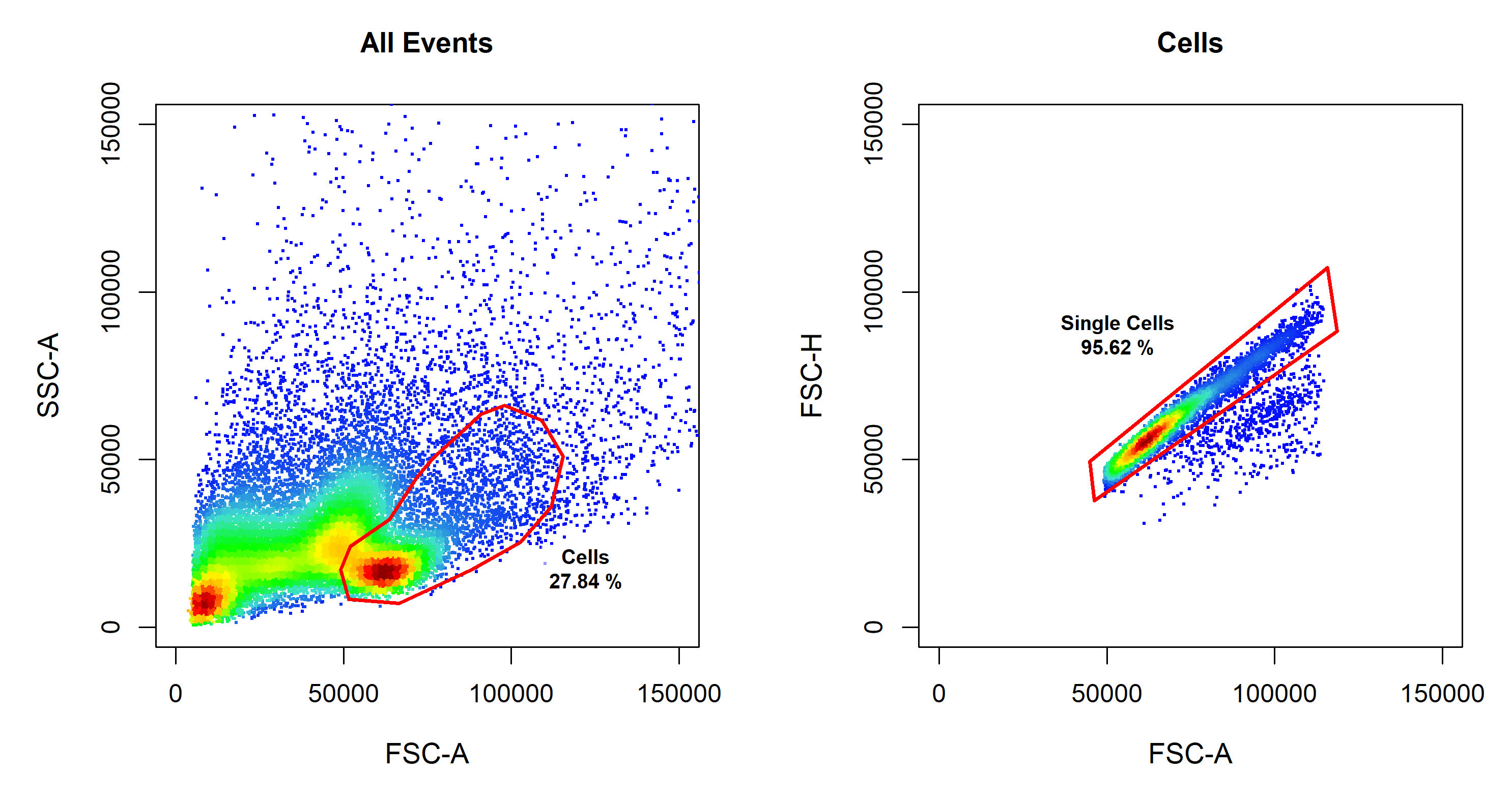
4.2 Compute Spillover Matrix
cyto_spillover_compute. Users are asked to assign a channel to compensation control and then gate the positive signal for each control in the indicated channel. CytoExploreR supports the use of either a universal unstained control or requires that each single colour control contain its own internal unstained reference population. The spillover matrix will be calculated using the method described by Bagwell & Adams 1993.
# Compute spillover matrix
spill <- cyto_spillover_compute(gs,
                                parent = "Single Cells",
                                spillover = "Spillover-Matrix.csv")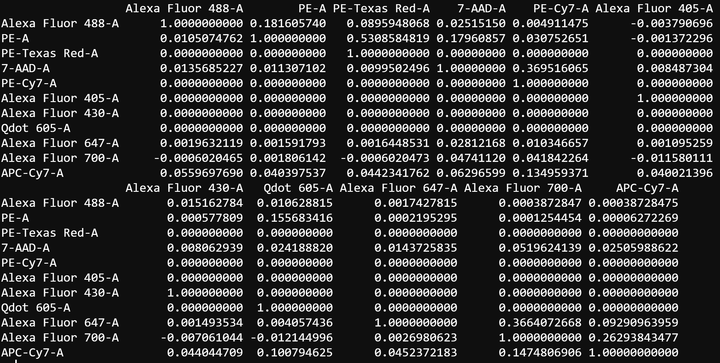
4.3 Edit Spillover Matrix
cyto_spillover_edit. Users should refer to the Plots to identify any lingering compensation issues and return to the Editor tab to refine the spillover matrix. By definition, the data is correctly compensated when the MedFI of the stained control is equal to that of the reference unstained control in all secondary detectors. The updated spillover matrix will be saved to a CSV file for downstream use.
# Edit spillover matrix
spill <- cyto_spillover_edit(gs,
                             parent = "Single Cells",
                             spillover = "Spillover-Matrix.csv")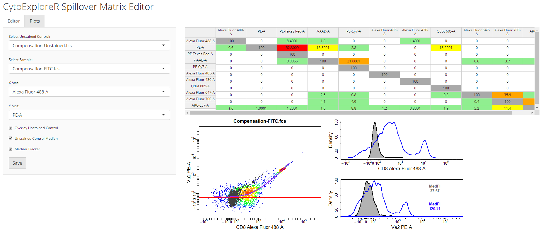
4.4 Visualise Compensation
cyto_plot_compensation. cyto_plot_compensation will plot uncompensated and compensated data in all fluorescent channels to check the compensation. The unstained control will automatically be overlaid onto the plots as a reference if supplied.
# Visualise uncompensated data
cyto_plot_compensation(gs,
                       parent = "Single Cells")

# Visualise compensated data
cyto_plot_compensation(gs,
                       parent = "Single Cells",
                       spillover = "Spillover-Matrix.csv",
                       compensate = TRUE)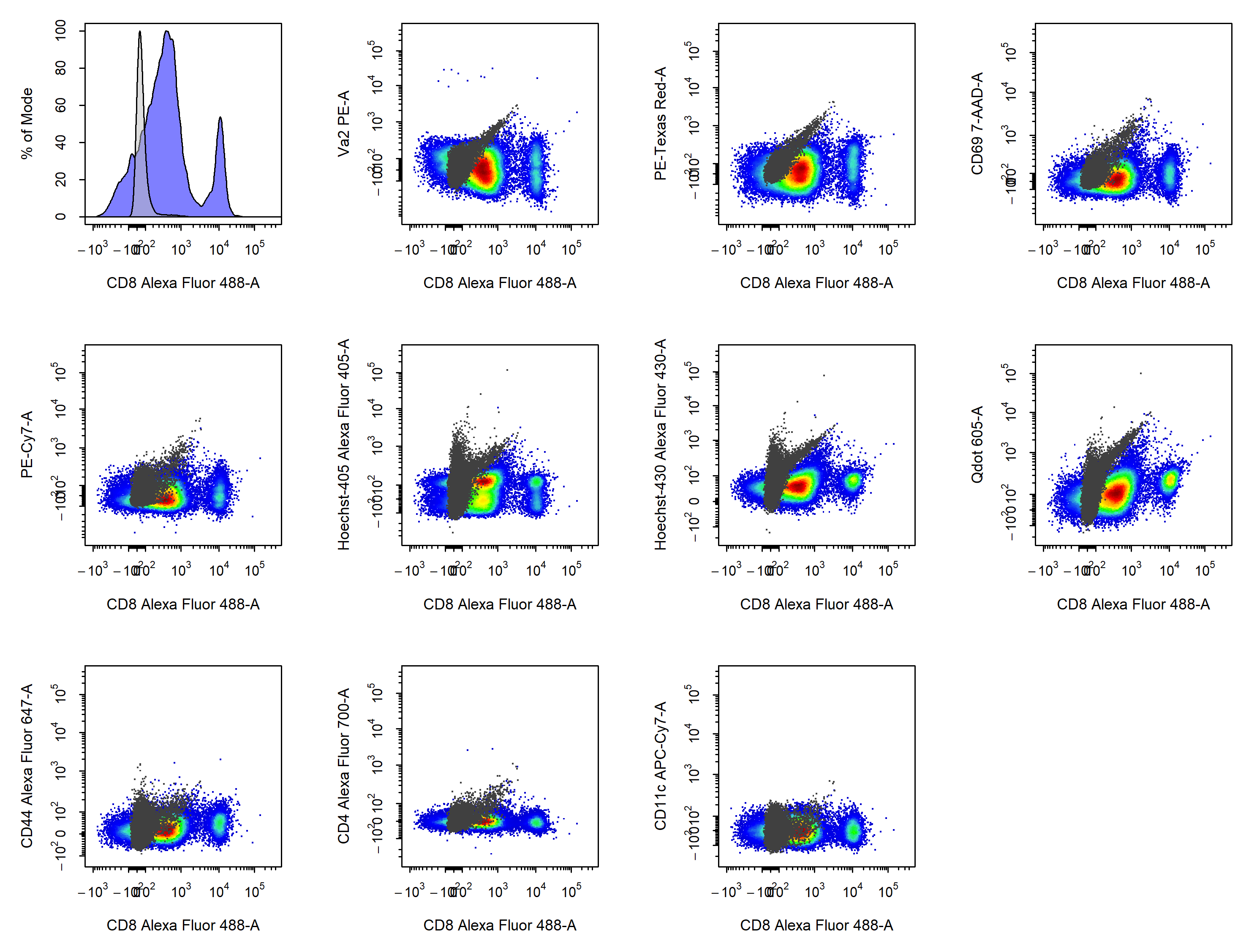
5. Analyse Samples
5.1 Load and Annotate Samples
cyto_setup. This function will open inteactive table editors to allow entry of experimenta markers and experiment details. For the purpose of demonstration, the details of this experiment have already been added.
# Load and annotate samples
gs <- cyto_setup("Activation-Samples",
                 gatingTemplate = "Activation-gatingTemplate.csv")
5.2 Apply Compensation and Data Transformations
cyto_compensate and transform the fluorescent channels using cyto_transform. It is important that data compensation and transformations occur in this order as compensation must be applied to linear data only.
# Apply compensation
gs <- cyto_compensate(gs,
                      spillover = "Spillover-Matrix.csv")

# Transform fluorescent channels - default logicle transformations
gs <- cyto_transform(gs)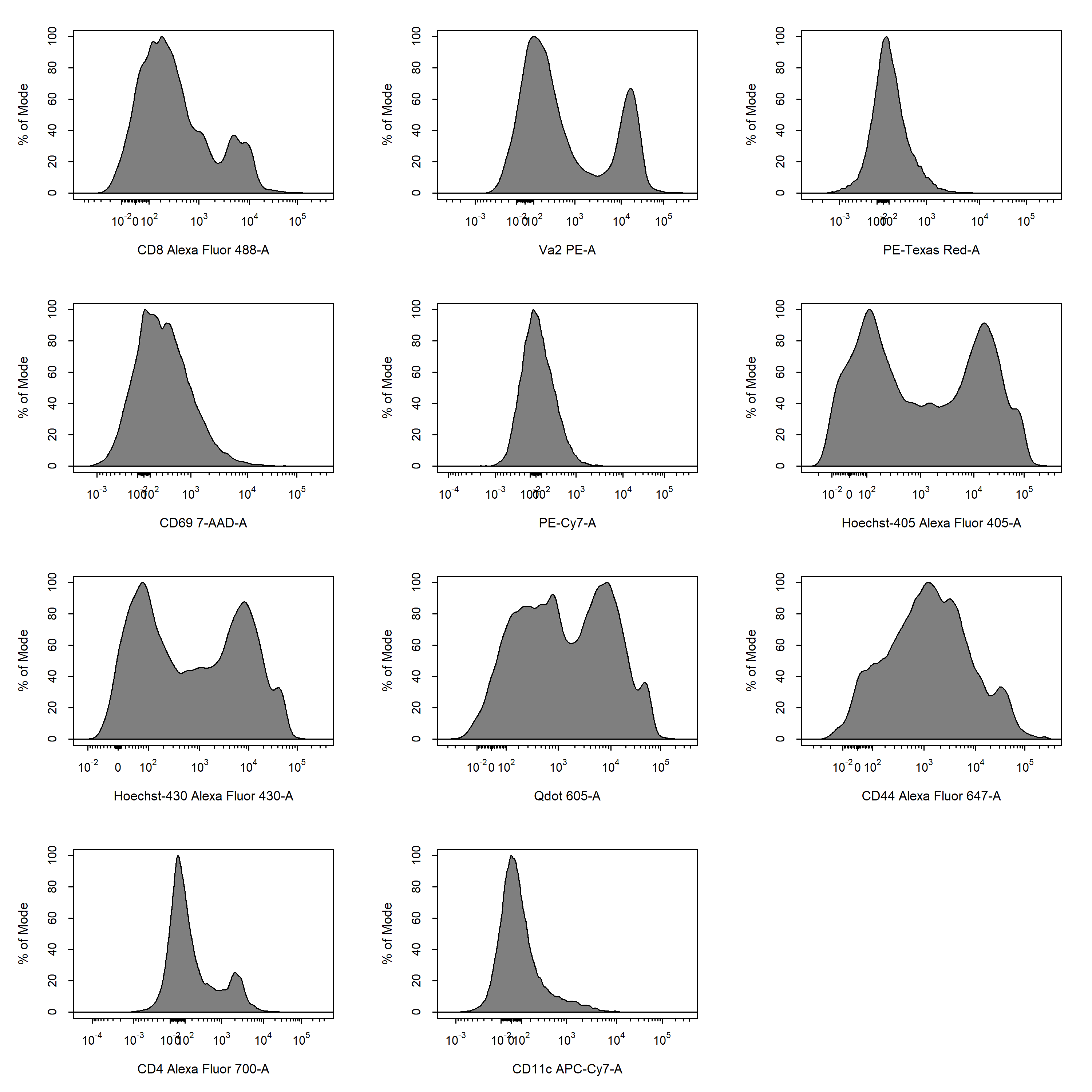
5.3 Gate Samples
cyto_gate_draw. This function allows us to interactively draw gates around populations using a variety of useful gate types. Let’s begin by drawing a polygon gate around the leukocyte population using the FSC-A and SSC-A parameteres. Since polygon gates are the default ate type for 2D plots, we don’t need to specify the gate type through the type argument. Polygon gates can be closed by right clicking and selecting “stop”.
# Gate Cells
cyto_gate_draw(gs,
               parent = "root",
               alias = "Cells",
               channels = c("FSC-A","SSC-A"))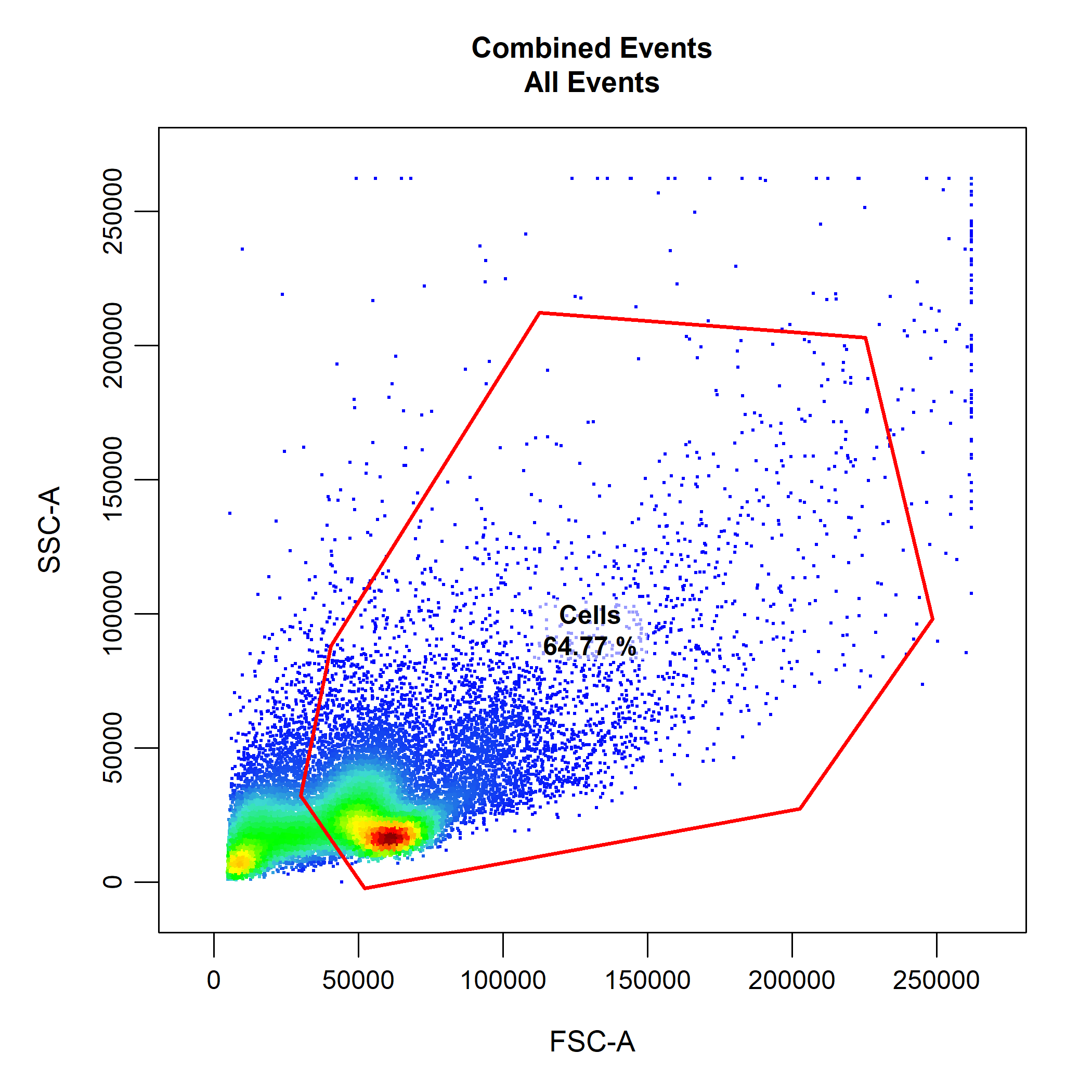
# Gate Single Cells
cyto_gate_draw(gs,
               parent = "Cells",
               alias = "Single Cells",
               channels = c("FSC-A","FSC-H"))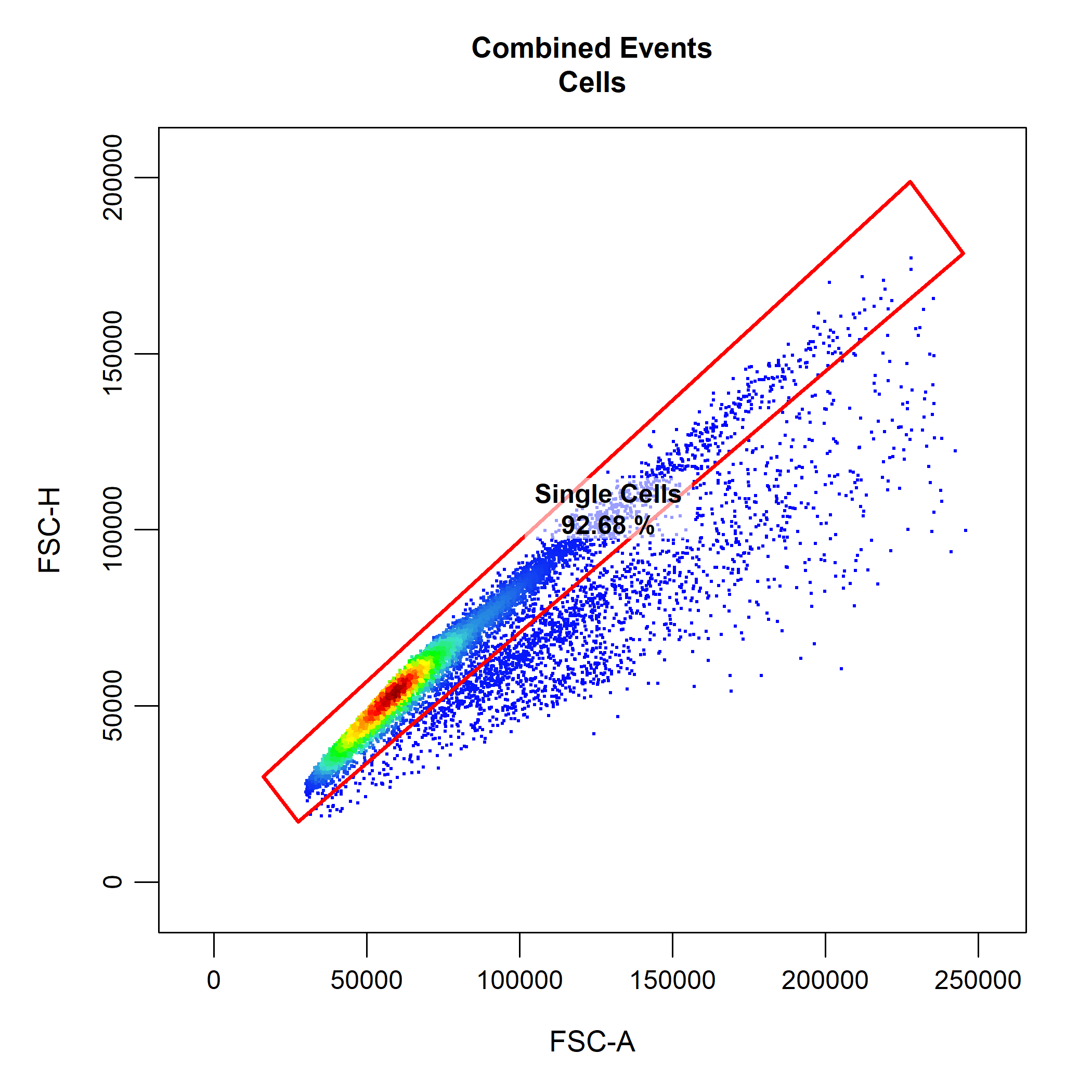
cyto_gate_draw makes use of cyto_plot to visualise the data. This means that we can pass any cyto_plot arguments through cyto_gate_draw to modify the constructed plots. This allows us to pull out samples or populations and overlay them on the plot to help us decide where the gate(s) should be set. As an examples, below we have extracted the unstained control and overlaid it onto the plot so that we can better set our live and dead cells gates. Notice how CytoExploreR supports gate negation through the negate argument. This means that any events outside the dead cells gate will be classified as live cells without the need for drawing additional gates. To construct the rectangle gate simply select the two diagonal points that encompass the population.
# Extract unstained control
NIL <- cyto_extract(gs, "Single Cells")[[33]]

# Gate Live Cells
cyto_gate_draw(gs,
               parent = "Single Cells",
               alias = c("Dead Cells", "Live Cells"),
               channels = c("Hoechst-405", "Hoechst-430"),
               type = "rectangle",
               negate = TRUE,
               overlay = NIL)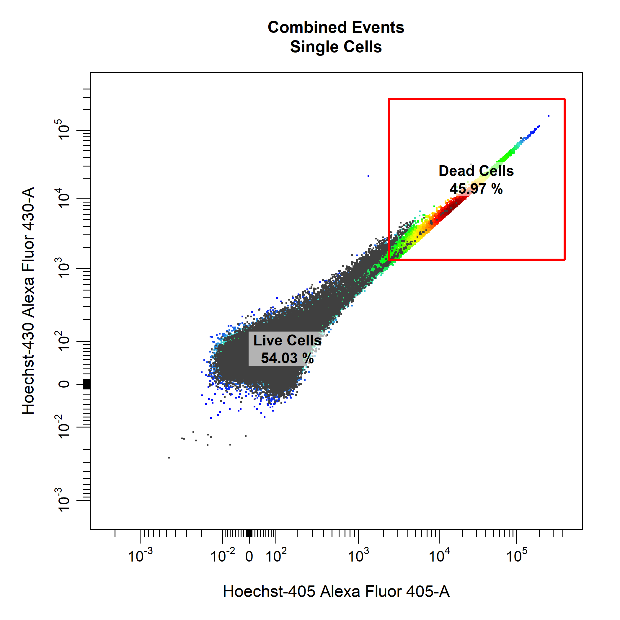
cyto_gate_draw also has support for mixed gate type when gating multiplpe populations. For example, we could use an ellipsoid gate for the T cells population and a rectangle gate for the dendritic cells populations.
# Gate T Cells and Dedritic Cells
cyto_gate_draw(gs,
               parent = "Live Cells",
               alias = c("T Cells", "Dendritic Cells"),
               channels = c("CD11c", "Va2"),
               type = c("ellipse", "rectangle"),
               overlay = NIL)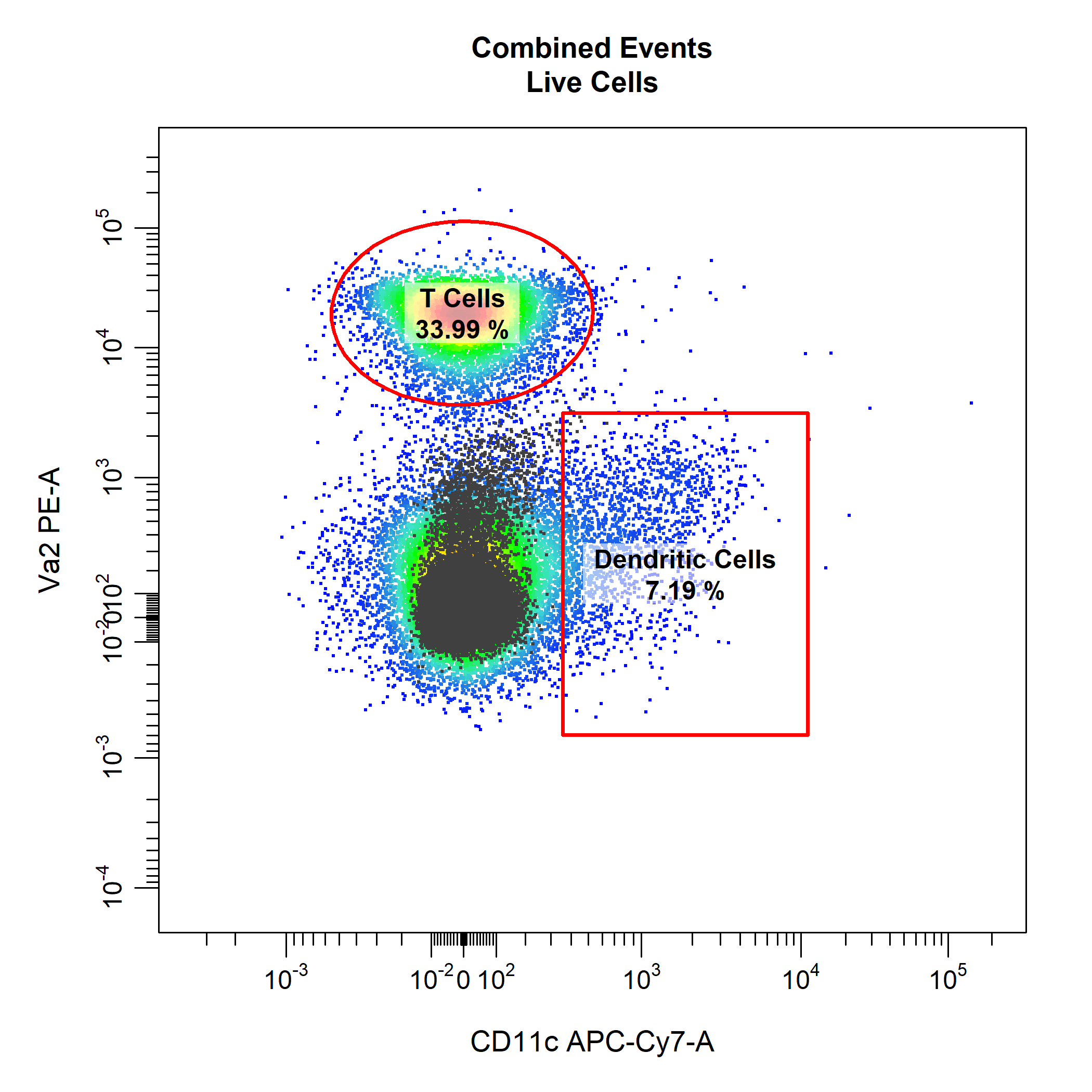
# Gate CD4 & CD8 T Cells
cyto_gate_draw(gs,
               parent = "T Cells",
               alias = c("CD4 T Cells", "CD8 T Cells"),
               channels = c("CD4", "CD8"),
               type = "r")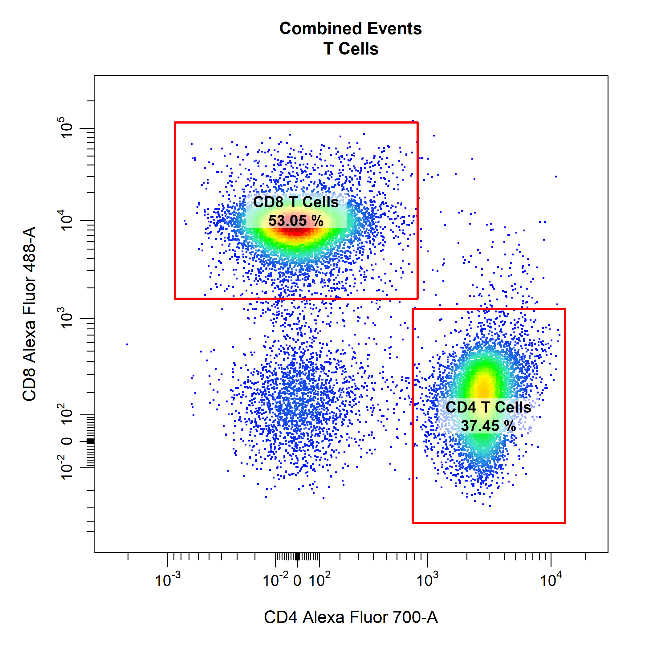
# Extract CD4 T Cells
CD4 <- cyto_extract(gs, "CD4 T Cells")

# Extract naive CD4 T Cells
CD4_naive <- cyto_select(CD4, OVAConc = 0)

# Gate CD69+ CD4 T Cells
cyto_gate_draw(gs,
               parent = "CD4 T Cells",
               alias = "CD69+ CD4 T Cells",
               channels = c("CD44", "CD69"),
               type = "rectangle",
               overlay = CD4_naive)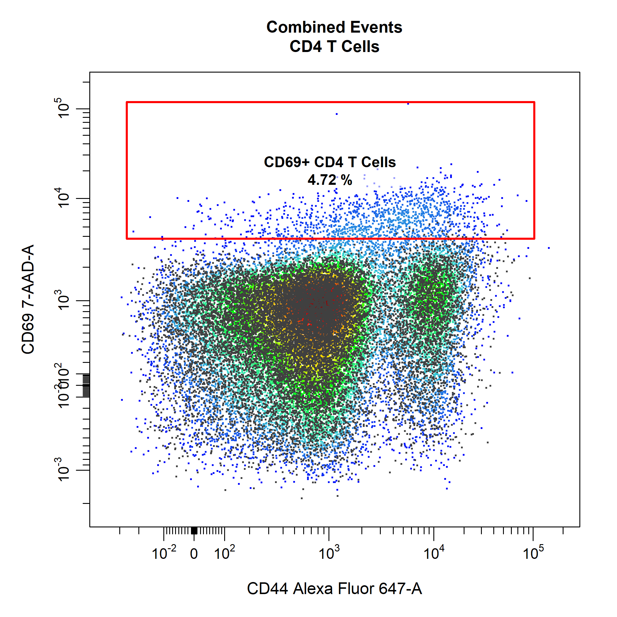
# Gate CD69+ CD8 T Cells
cyto_gate_draw(gs,
               parent = "CD8 T Cells",
               alias = "CD69+ CD8 T Cells",
               channels = c("CD44", "CD69"),
               type = "rectangle",
               contour_lines = 15)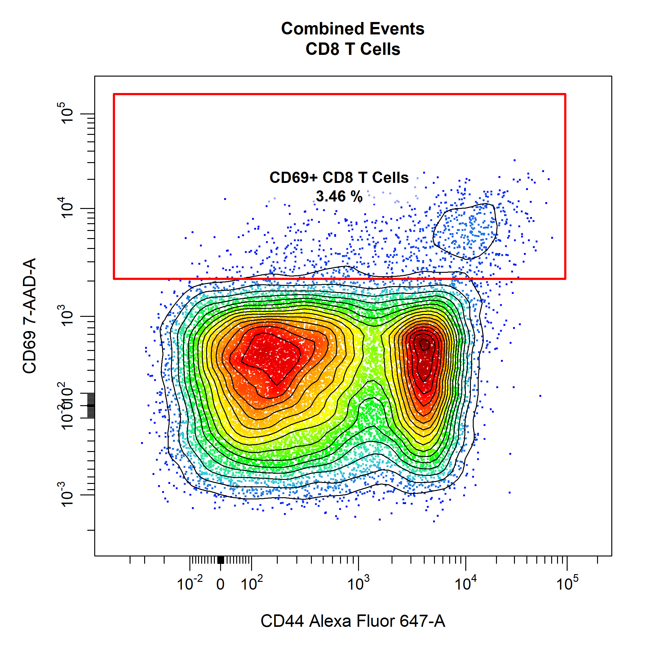
5.4 Explore Gated Samples
cyto_plot_gating_tree. This function plots the gating tree with nodes scaled by population size and can also display frequency and count statistics for each node. Since cyto_plot_gating_tree doesn’t plot the actual data it is super fast and provides a quick overview of the data. It is also completely interactive! Try clicking and dragging nodes, it’s loads of fun!
# Gating Tree
cyto_plot_gating_tree(gs[[32]],
stat = "freq")cyto_plot_gating_scheme. This is an extremely powerful function that can plot gating schemes for all samples, and has full support for back gating and gate tracking.
# Gating scheme
cyto_plot_gating_scheme(gs[32],
                        back_gate = TRUE,
                        gate_track = TRUE)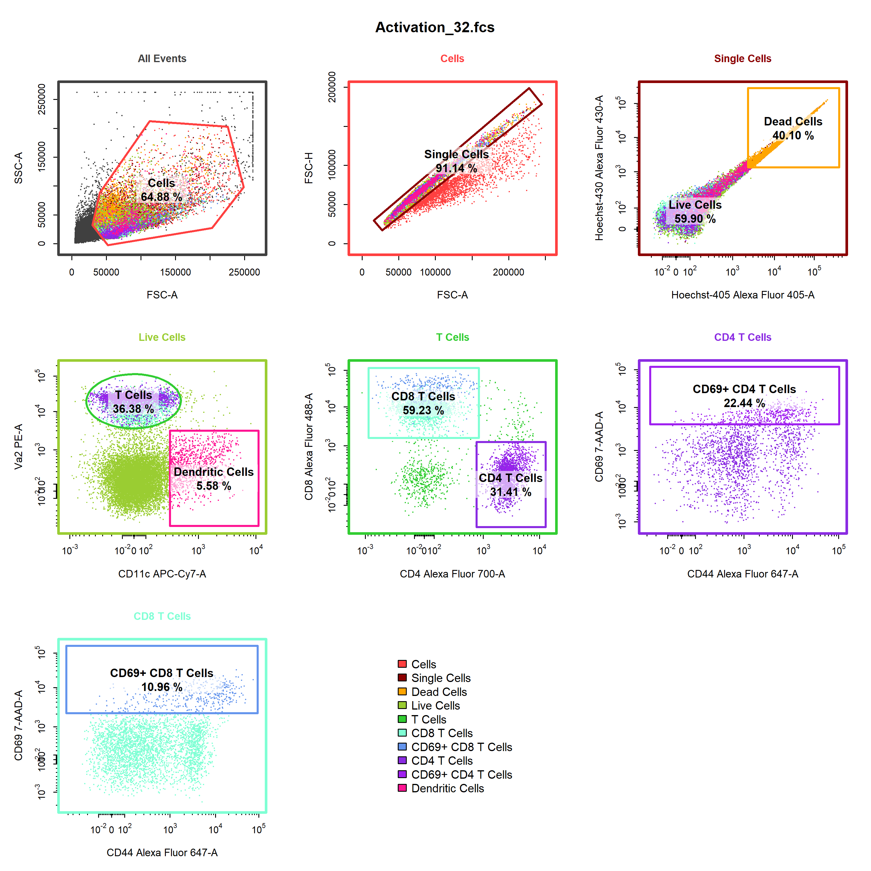
5.5 Export Statistics
cyto_stats_compute which will compute the desired statistics for the specified populations and return a tidyverse friendly output that retains all the experiment details. This makes it easy to plot the exported statistics using other R packages, such as ggplot2.
# Compute medFI - exclude unstained control
cyto_stats_compute(gs[1:32],
                   alias = c("CD69+ CD4 T Cells",
                             "CD69+ CD8 T Cells"),
                   stat = "median",
                   channels = c("CD44", "CD69"))
#> # A tibble: 128 x 6
#>    name             OVAConc Treatment Population        Marker  MedFI
#>    <fct>            <chr>   <chr>     <chr>             <chr>   <dbl>
#>  1 Activation_1.fcs 0       Stim-A    CD69+ CD4 T Cells CD44   18695.
#>  2 Activation_1.fcs 0       Stim-A    CD69+ CD8 T Cells CD44    3523.
#>  3 Activation_1.fcs 0       Stim-A    CD69+ CD4 T Cells CD69    4315.
#>  4 Activation_1.fcs 0       Stim-A    CD69+ CD8 T Cells CD69    2579.
#>  5 Activation_2.fcs 0       Stim-A    CD69+ CD4 T Cells CD44   13892.
#>  6 Activation_2.fcs 0       Stim-A    CD69+ CD8 T Cells CD44    2559.
#>  7 Activation_2.fcs 0       Stim-A    CD69+ CD4 T Cells CD69    4298.
#>  8 Activation_2.fcs 0       Stim-A    CD69+ CD8 T Cells CD69    2783.
#>  9 Activation_3.fcs 5       Stim-A    CD69+ CD4 T Cells CD44   15815.
#> 10 Activation_3.fcs 5       Stim-A    CD69+ CD8 T Cells CD44    2826.
#> # ... with 118 more rows