
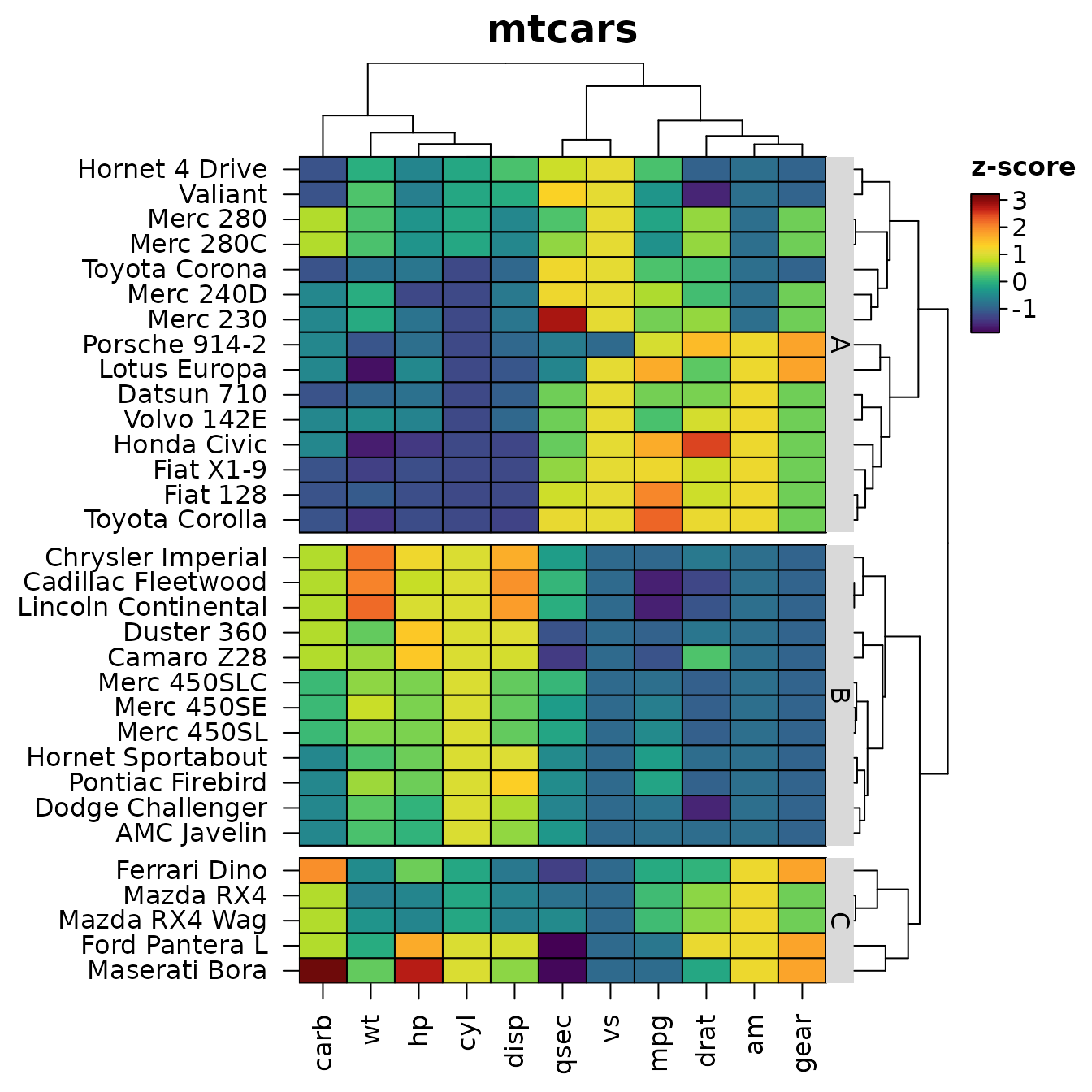
heat_map() draws a heatmap and returns it as an object.
This article shows what you can do with that object: redraw it with
changes, save it, take its orders and clusters for further analysis,
rebuild it in ggplot2, place it beside ggplot2
plots, and describe it in words for readers who can’t see it.
library(HeatmapR)
hm <- heat_map(
  mtcars,
  scale = "zscore",
  tree = "both",
  tree_cut_y = 3,
  tree_label_y = TRUE,
  tree_label_text_y = c("A", "B", "C"),
  legend_title = "z-score",
  title = "mtcars"
)
Redrawing and saving
A heat_map object is the recordedplot of
the heatmap together with the arguments that made it.
print() and plot() draw it again, with any
argument replaced, and data draws other data with the same
settings. The slow steps (dendrograms, k-means clusters, branch support)
are reused when nothing they depend on has changed, so a redraw only
draws.
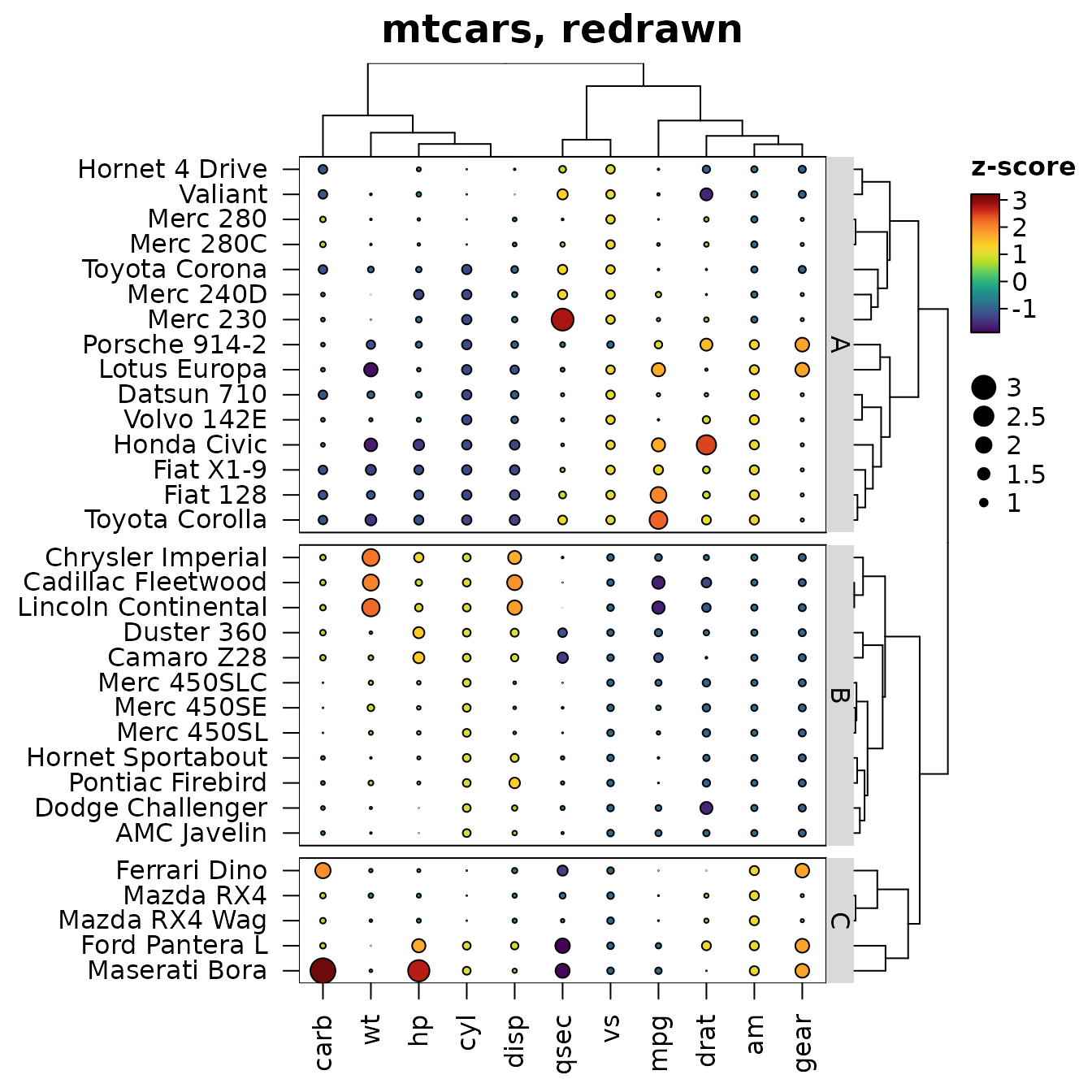
heat_map_save() writes a heatmap to a file (PNG, JPEG,
TIFF, PDF or SVG, from the extension), at the size and resolution you
choose: either the object itself (x = hm) or every heatmap
drawn after the call until heat_map_complete().
file <- tempfile(fileext = ".pdf")
heat_map_save(file, x = hm, width = 6, height = 7)
file.exists(file)
#> [1] TRUE
Styles
heat_map_style() keeps settings of
heat_map() - colour scales, text sizes, borders, legend
options - to reuse across heatmaps, so the figures of a report or paper
look alike without repeating a dozen arguments. A style given to
style fills in the arguments that aren’t given, and
options(HeatmapR.style = ) gives every heatmap of the
session the style, including dot plots, correlation and aligned
heatmaps. Styles build on styles, and redrawn heatmaps keep the style
they were drawn with:
paper <- heat_map_style(
  cell_col_scale = "Blue-Red 3",
  cell_col_scale_center = 0,
  cell_border_line_col = "white",
  axis_text_size_x = 0.8,
  axis_text_size_y = 0.8,
  legend_side = "bottom"
)
paper
#> A heat_map() style with 6 settings:
#>   cell_col_scale = "Blue-Red 3"
#>   cell_col_scale_center = 0
#>   cell_border_line_col = "white"
#>   axis_text_size_x = 0.8
#>   axis_text_size_y = 0.8
#>   legend_side = "bottom"
heat_map(mtcars, scale = "zscore", tree = "both", style = paper,
         title = "mtcars, styled")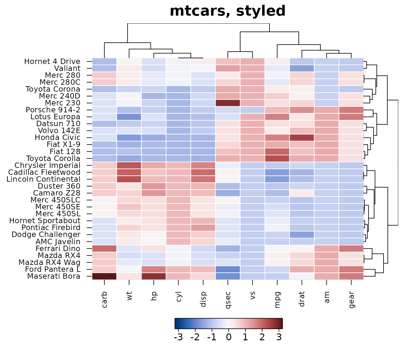
Orders, clusters and colours
heat_map_info() returns what the heatmap is made of: the
data as displayed (after scaling), the order of the rows and columns,
the cluster of each row and column, the dendrograms, the colour, size
and shape of every cell, and the bounding box of every component in
inches.
info <- heat_map_info(hm)
names(info)
#>  [1] "data"          "row_order"     "col_order"     "row_clusters"
#>  [5] "col_clusters"  "tree_x"        "tree_y"        "support_x"
#>  [9] "support_y"     "zoom_x"        "zoom_y"        "axis_text_x"
#> [13] "axis_text_y"   "colours"       "split_colours" "split_sizes"
#> [17] "split_data"    "bimodal"       "sizes"         "shapes"
#> [21] "centers"       "annotations"   "layout"        "raster"
#> [25] "col_limits"    "col_blocks"    "size_limits"   "keys"
#> [29] "scales"
# THE ROWS IN THE ORDER THEY ARE SHOWN, FROM THE TOP
head(rownames(mtcars)[info$row_order])
#> [1] "Hornet 4 Drive" "Valiant"        "Merc 280"       "Merc 280C"
#> [5] "Toyota Corona"  "Merc 240D"
# THE CLUSTER OF EACH CAR
split(rownames(mtcars), info$row_clusters)
#> $`1`
#>  [1] "Datsun 710"     "Hornet 4 Drive" "Valiant"        "Merc 240D"
#>  [5] "Merc 230"       "Merc 280"       "Merc 280C"      "Fiat 128"
#>  [9] "Honda Civic"    "Toyota Corolla" "Toyota Corona"  "Fiat X1-9"
#> [13] "Porsche 914-2"  "Lotus Europa"   "Volvo 142E"
#>
#> $`2`
#>  [1] "Hornet Sportabout"   "Duster 360"          "Merc 450SE"
#>  [4] "Merc 450SL"          "Merc 450SLC"         "Cadillac Fleetwood"
#>  [7] "Lincoln Continental" "Chrysler Imperial"   "Dodge Challenger"
#> [10] "AMC Javelin"         "Camaro Z28"          "Pontiac Firebird"
#>
#> $`3`
#> [1] "Mazda RX4"      "Mazda RX4 Wag"  "Ford Pantera L" "Ferrari Dino"
#> [5] "Maserati Bora"
info$layout[1:4, ]
#>   component     xmin     xmax      ymin  ymax
#> 1   heatmap 1.916527 5.296403 0.6968001 5.995
#> 2    tree_x 1.916527 5.296403 5.9950000 6.595
#> 3  labels_y 5.296403 5.476090 0.6968001 5.995
#> 4    tree_y 5.476090 6.076090 0.6968001 5.995
The clusters are numbered from the top of the heatmap, as they are labelled, so they can be used straight away, e.g. to compare the cars of each cluster:
Tidy data for ggplot2
heat_map_data() returns what the heatmap shows as tidy
tables: one row per cell, row, column or dendrogram segment.
x and y are the centres of the cells in the
heatmap’s own co-ordinates, including the gaps between clusters, so a
heatmap can be rebuilt or restyled with ggplot2, exported,
or drawn on with base graphics.
cells <- heat_map_data(hm)
head(cells)
#>              row column row_index col_index display_row display_col   x
#> 1 Hornet 4 Drive   carb         4        11           1           1 0.5
#> 2 Hornet 4 Drive     wt         4         6           1           2 1.5
#> 3 Hornet 4 Drive     hp         4         4           1           3 2.5
#> 4 Hornet 4 Drive    cyl         4         2           1           4 3.5
#> 5 Hornet 4 Drive   disp         4         3           1           5 4.5
#> 6 Hornet 4 Drive   qsec         4         7           1           6 5.5
#>          y        value    colour size shape row_cluster
#> 1 32.49656 -1.122152071 #3A538AFF    1  rect           1
#> 2 32.49656 -0.002299538 #2AAF7FFF    1  rect           1
#> 3 32.49656 -0.535092840 #24858DFF    1  rect           1
#> 4 32.49656 -0.104987809 #25A783FF    1  rect           1
#> 5 32.49656  0.220093694 #4AC16DFF    1  rect           1
#> 6 32.49656  0.890487156 #CCDE29FF    1  rect           1
library(ggplot2)
rows <- heat_map_data(hm, "rows")
cols <- heat_map_data(hm, "columns")
tree <- heat_map_data(hm, "tree_y")
edge <- max(cells$x) + 0.5
grow <- function(h) edge + 3 * h / max(tree$x)
ggplot(cells) +
  geom_tile(aes(x, y, fill = value), colour = "white") +
  geom_segment(data = tree, aes(x = grow(x), y = y, xend = grow(xend), yend = yend)) +
  scale_fill_distiller(palette = "RdBu", name = "z-score") +
  scale_x_continuous(breaks = cols$x, labels = cols$column) +
  scale_y_continuous(breaks = rows$y, labels = rows$row) +
  labs(x = NULL, y = NULL) +
  theme_minimal() +
  theme(panel.grid = element_blank(),
        axis.text.x = element_text(angle = 90, hjust = 1, vjust = 0.5))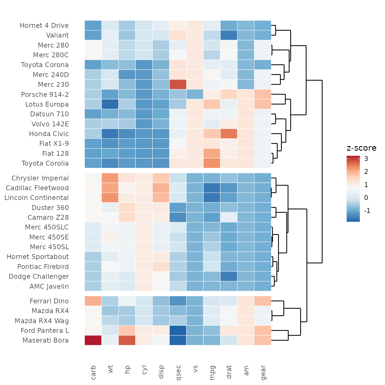
Drawn straight after heat_map(), base graphics land on
the cells. Below, the largest value in each column is marked with a
star:
hm <- heat_map(mtcars, scale = "zscore", tree = "both", legend_title = "z-score")
cells <- heat_map_data(hm)
top <- cells[ave(cells$value, cells$column, FUN = max) == cells$value, ]
points(top$x, top$y, pch = 8, col = "white", cex = 1.5)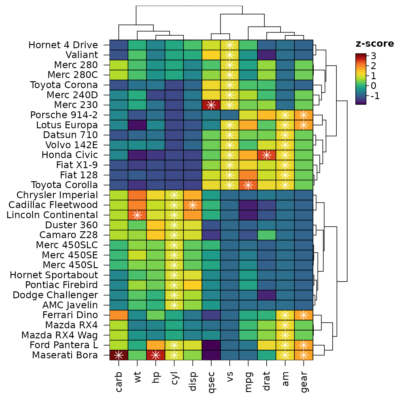
Beside ggplot2 plots
heat_map_grob() turns a heatmap into a grid
graphical object, so it can sit beside ggplot2 plots in
patchwork, cowplot or gridExtra
layouts. The grob draws the heatmap again whenever its space changes, so
dendrograms, legends and text are sized for the space it is given. It
needs the gridGraphics package.
library(patchwork)
p <- ggplot(mtcars, aes(wt, mpg, colour = factor(cyl))) +
  geom_point(size = 2) +
  labs(x = "Weight (1000 lbs)", y = "Miles per gallon", colour = "Cylinders") +
  theme_bw()
p + heat_map_grob(hm, title = "mtcars") + plot_layout(widths = c(1, 1.5))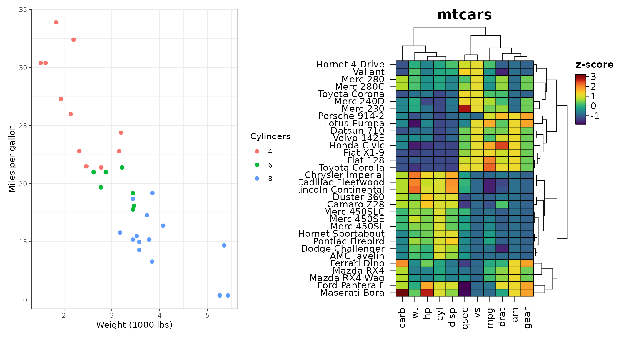
Several heatmaps can also share one figure with
heat_map_custom(), which takes a layout (a number of rows
and columns, or a matrix as in graphics::layout()), and
heat_map_complete() to finish it.
heat_map_custom(popup = FALSE, layout = c(1, 3))
heat_map(mtcars[grepl("Merc", rownames(mtcars)), ], scale = "column",
         legend = FALSE, title = "Mercedes")
heat_map(mtcars[grepl("Mazda|Toyota", rownames(mtcars)), ], scale = "column",
         legend = FALSE, title = "Mazda | Toyota")
heat_map(mtcars[grepl("Hornet|Datsun|Volvo", rownames(mtcars)), ],
         scale = "column", legend = FALSE, title = "Hornet | Datsun | Volvo")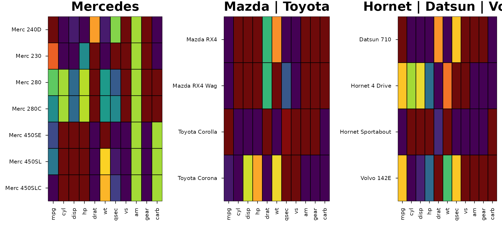
Heatmaps drawn on their own each have their own colour scale, so one
colour can stand for different values in each.
heat_map_arrange() redraws heatmaps in one layout on shared
colour limits (and cell size limits), from the lowest to the highest
limit of them all, and keeps their dendrograms and other settings:
merc <- heat_map(mtcars[grepl("Merc", rownames(mtcars)), ], title = "Mercedes")
others <- heat_map(mtcars[!grepl("Merc", rownames(mtcars)), ],
                   title = "The other cars")
heat_map_arrange(merc, others)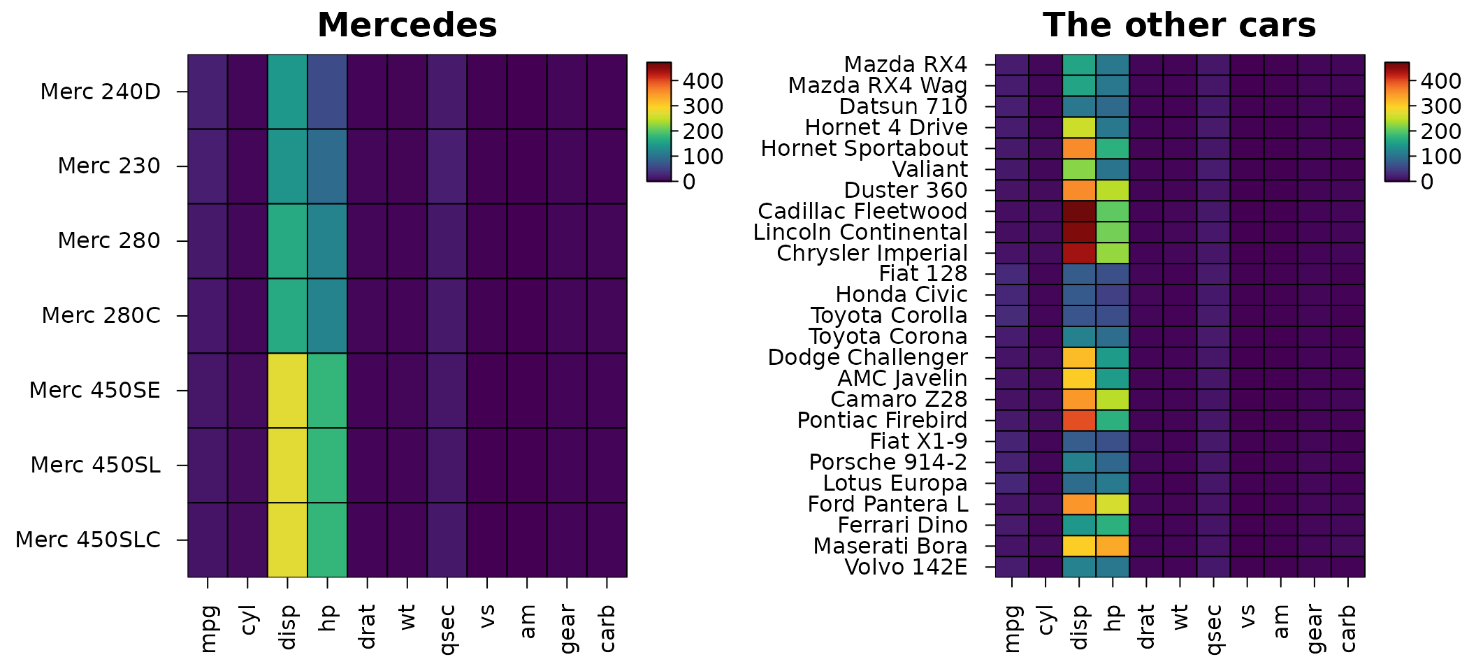
Interactive heatmaps
heat_map_html() turns a heatmap into a web page to
explore it: hovering over a cell shows its row, column and value (before
and after scaling, with its clusters and annotations); clicking a cell
or a label selects its row or column, and dragging a box across cells,
labels or a dendrogram selects every row and column in it, e.g. the
genes of a cluster; the selection can be copied, one name per line, or
downloaded with its values as a CSV file; a search box finds rows and
columns by name, and the heatmap zooms. The page is a single HTML file
with the heatmap as an SVG image, nothing to install and nothing loaded
from the web, so it works offline and can be shared by email. It opens
in the RStudio or Positron viewer (or a browser) from the console, and
in R Markdown and Quarto it is embedded where it is printed:
page <- heat_map_html(mtcars, scale = "column", tree = "both", tree_cut_y = 3,
                      legend_title = "Scaled", title = "mtcars", height = 6)
page
Any heatmap can be given,
e.g. heat_map_html(heat_map_dot(...)), or data with the
arguments of heat_map(), as above.
Building heatmaps in the browser
heat_map_app() opens an app to build heatmaps, dot plots
and correlation heatmaps without writing code. You can drop a table or a
single-cell file on it, or start it from data in R. It redraws the
heatmap as settings change, shows values on hover and selects rows and
columns on the heatmap, and writes the R code that draws the figure
again:
heat_map_app()                             # the start page: drop a file or choose an example
heat_map_app(mtcars, scale = "column")     # start from data in R, with settings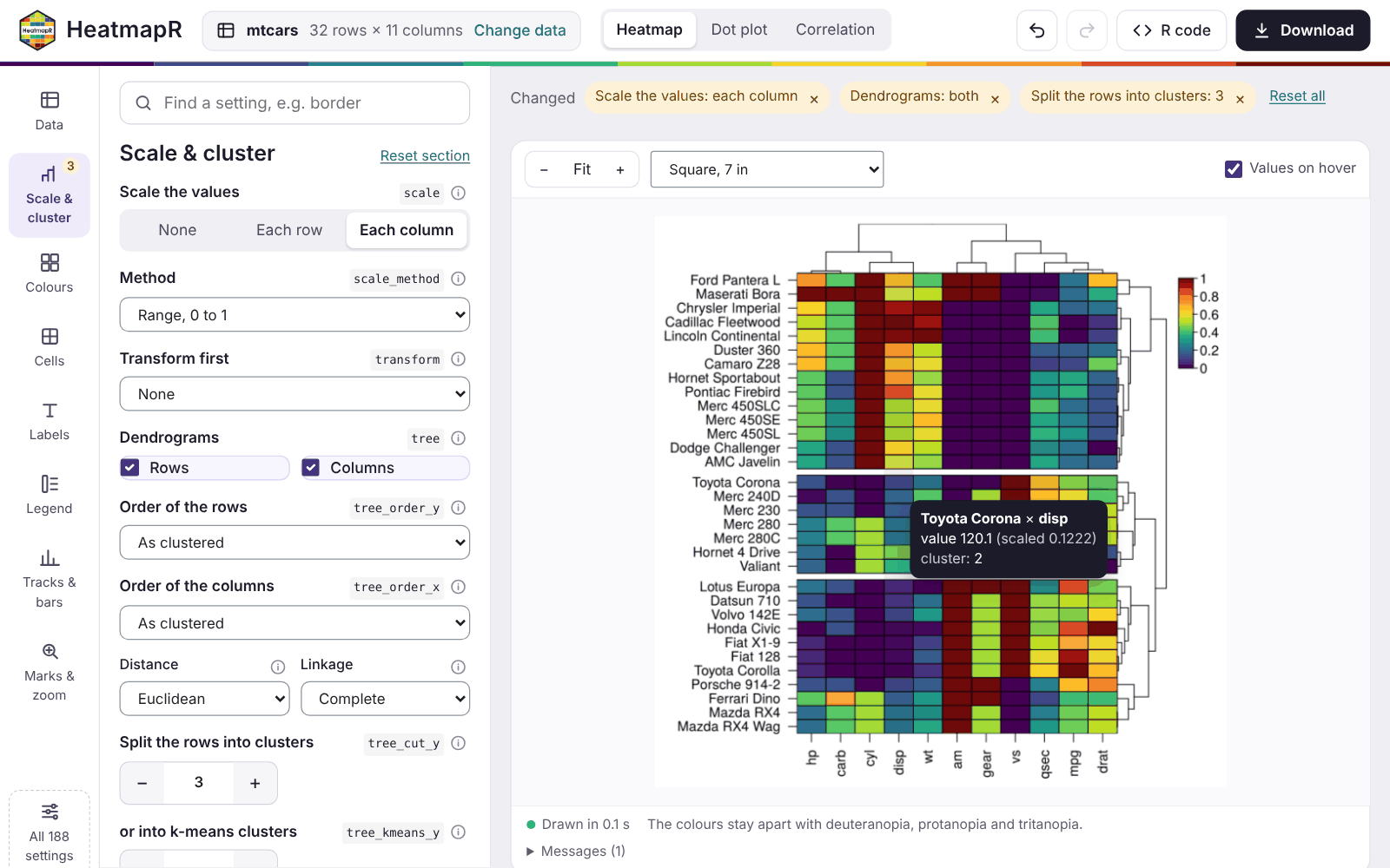
Building heatmaps in the browser walks through the app: its data, plots, settings, selections, code and downloads, and hosting it for others.
Alternative text
Figures in reports and on the web need alternative text for readers
using screen readers, and a heatmap is hard to describe by hand.
heat_map_describe() writes the description from the heatmap
itself: its size and scaling, what the colours show (naming the colours
of the scale), the most extreme values, how the rows and columns are
ordered, and where each cluster is highest and lowest, plus branch
support, uncertainty, annotations, bars and zoom panels when the heatmap
has them.
hm <- heat_map(mtcars, scale = "zscore", tree = "both", tree_cut_y = 3,
               legend_title = "z-score", title = "mtcars")
heat_map_describe(hm)
#> Heatmap titled "mtcars" of 32 rows by 11 columns, converted to z-scores within
#> each column. Colours show z-score, from dark purple (-1.87) through yellow
#> green to dark red (3.21). The highest value is 3.21 (Maserati Bora, carb) and
#> the lowest is -1.87 (Ford Pantera L, qsec). Rows are ordered by hierarchical
#> clustering (euclidean distance, complete linkage). Rows are split into 3
#> groups, numbered from the top: group 1 (15 rows, e.g. Hornet 4 Drive and
#> Valiant) is highest in vs and mpg and lowest in cyl and hp; group 2 (12 rows,
#> e.g. Chrysler Imperial and Cadillac Fleetwood) is highest in disp and cyl and
#> lowest in gear and drat; group 3 (5 rows, e.g. Ferrari Dino and Mazda RX4) is
#> highest in carb and gear and lowest in qsec and vs. Columns are ordered by
#> hierarchical clustering (euclidean distance, complete linkage).
In R Markdown and Quarto the description can be the figure’s
alternative text: draw the heatmap in one chunk and pass the description
to the fig.alt option of the chunk that shows it.
```{r, include = FALSE}
hm <- heat_map(mtcars, scale = "zscore", tree = "both", tree_cut_y = 3)
```

```{r, fig.alt = heat_map_describe(hm)}
hm
```
hm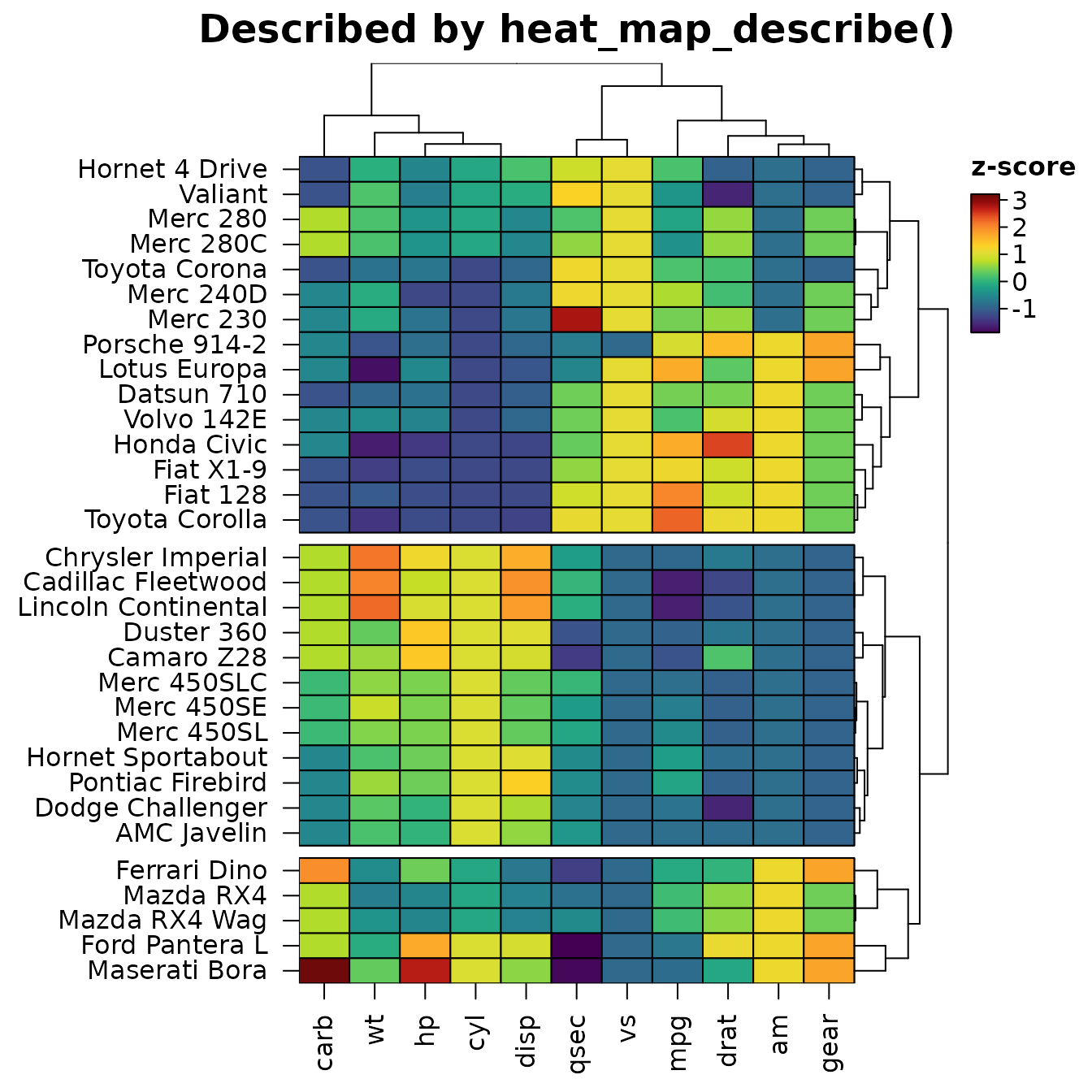
Colour-blind readers
About one man in twelve of northern European descent has a red-green
colour-vision deficiency. heat_map_check_colours()
simulates how a heatmap’s colours look with deuteranopia, protanopia and
tritanopia (as Machado et al. 2009 model them) and lists the annotation
levels, values of non-numeric cells, stacked bar parts and branch
colours that become hard to tell apart, and colour scales whose distant
values end up looking alike. Here matplotlib’s red and green, which most
readers tell apart easily, are close for readers with deuteranopia:
cylinders <- data.frame(cylinders = factor(mtcars$cyl), row.names = rownames(mtcars))
hm <- heat_map(mtcars, scale = "column", annotation_y = cylinders,
               annotation_colours = list(cylinders = c("#D62728", "#2CA02C", "#1F77B4")))
heat_map_check_colours(hm)
#> 1 pair of colours is hard to tell apart (annotation cylinders), e.g. 4 and 6 of annotation cylinders with deuteranopia. The first eight colours of palette.colors(palette = "Okabe-Ito") stay apart for colour-blind readers.
#>
#> annotation cylinders:
#>   4 and 6 (deuteranopia, Delta E 7.3)
options(HeatmapR.check_colours = TRUE) checks every
heatmap as it is drawn, with a message when colours are hard to tell
apart. The first eight colours of
palette.colors(palette = "Okabe-Ito") stay apart for each
deficiency, and the default colour scale changes in lightness from end
to end, so its values stay readable.