Overview
HeatmapR is a lightweight R package that uses base
graphics to facilitate the creation of high quality complex heatmaps
that can be easily arranged with other plots. In this vignette, we will
explore the key features of HeatmapR and describe the usage
of each of the key functions in HeatmapR as summarised
below:
-
heat_map()convenient wrapper around allHeatmapRfunctions providing an intuitive way to create complex heatmaps using base graphics. -
heat_map_clust()is used insideheat_map()to perform hierarchical clustering on the dataset usingstats::hclust(). -
heat_map_scale()is used insideheat_map()to apply column- or row-wise mean, z-score or range scaling to the dataset prior to constructing the heatmap. -
heat_map_layout()allows you to create custom plot layouts to arrange multiple heatmaps. -
heat_map_save()can be called prior to anyheat_map()call to save a high resolution image. -
heat_map_record()can be called after anyheat_map()calls to record the current plot for saving to an R object. -
heat_map_complete()can be called when creating complex layouts to indicate when the resulting layout should be saved to file usingheat_map_save(). -
heat_map_reset()resets all HeatmapR associated settings in case things are not working as they should.
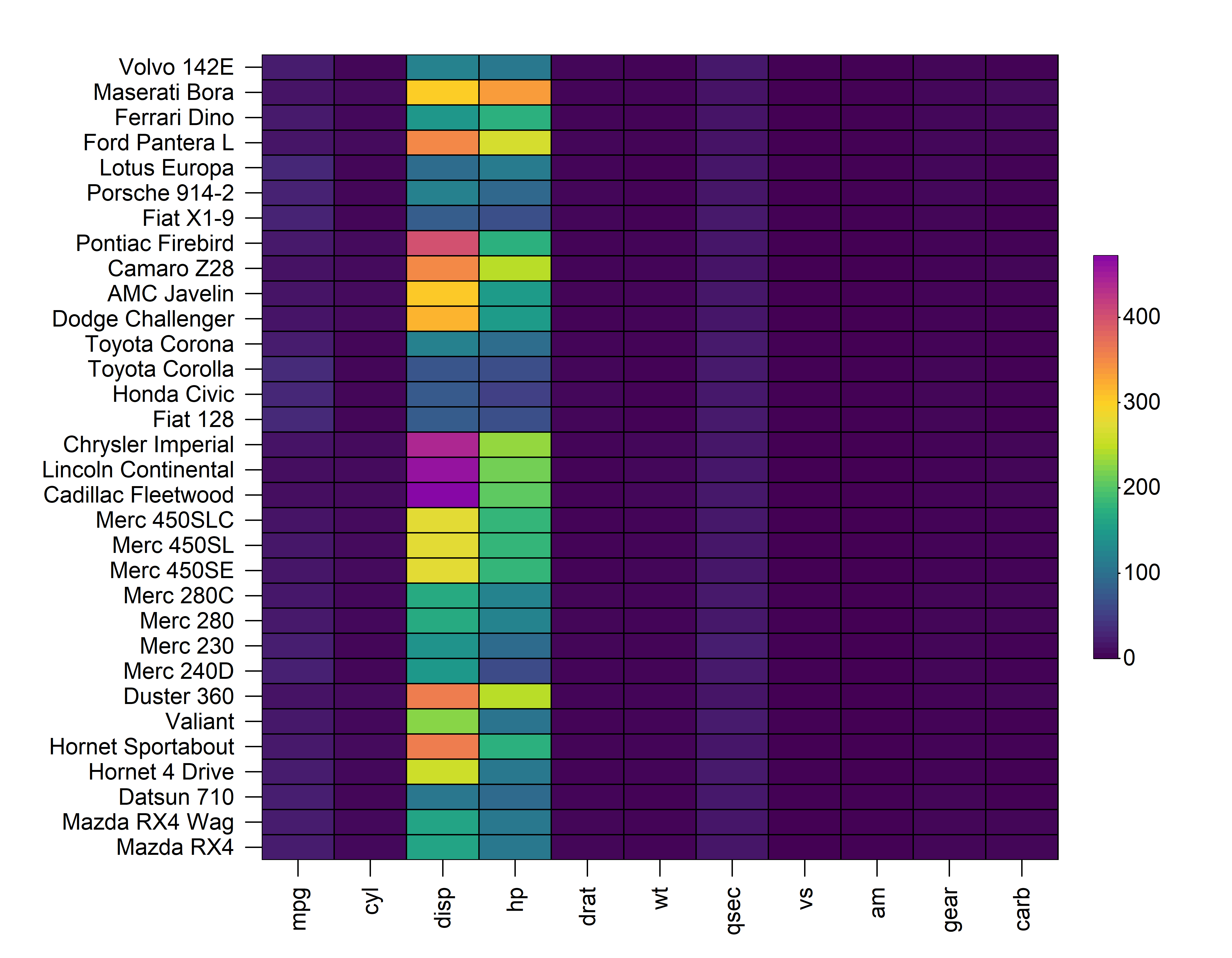
1. Construct a Basic Heatmap
Constructing a heatmap is as simple loading the
HeatmapR package and supplying your dataset to the
heat_map() function. The constructed heatmap will be in the
same orientation as the input data and each numeric cell in the heatmap
will be coloured using the colour scale supplied to
cell_col_scale. By default, heat_map() uses a
hybrid colour blind friendly viridis palette to offer high
visual contrast.
2. Cell Properties
heat_map() contains a family of cell_
arguments which allow for the customisation of the shape, size, colour,
borders and text of cells within a heatmap. In the examples below, we
will apply the same properties to every cell within the heatmap, but it
is also possible to modify these properties per cell by supplying a
matrix matching the dimensionality and orientation of the input
matrix.
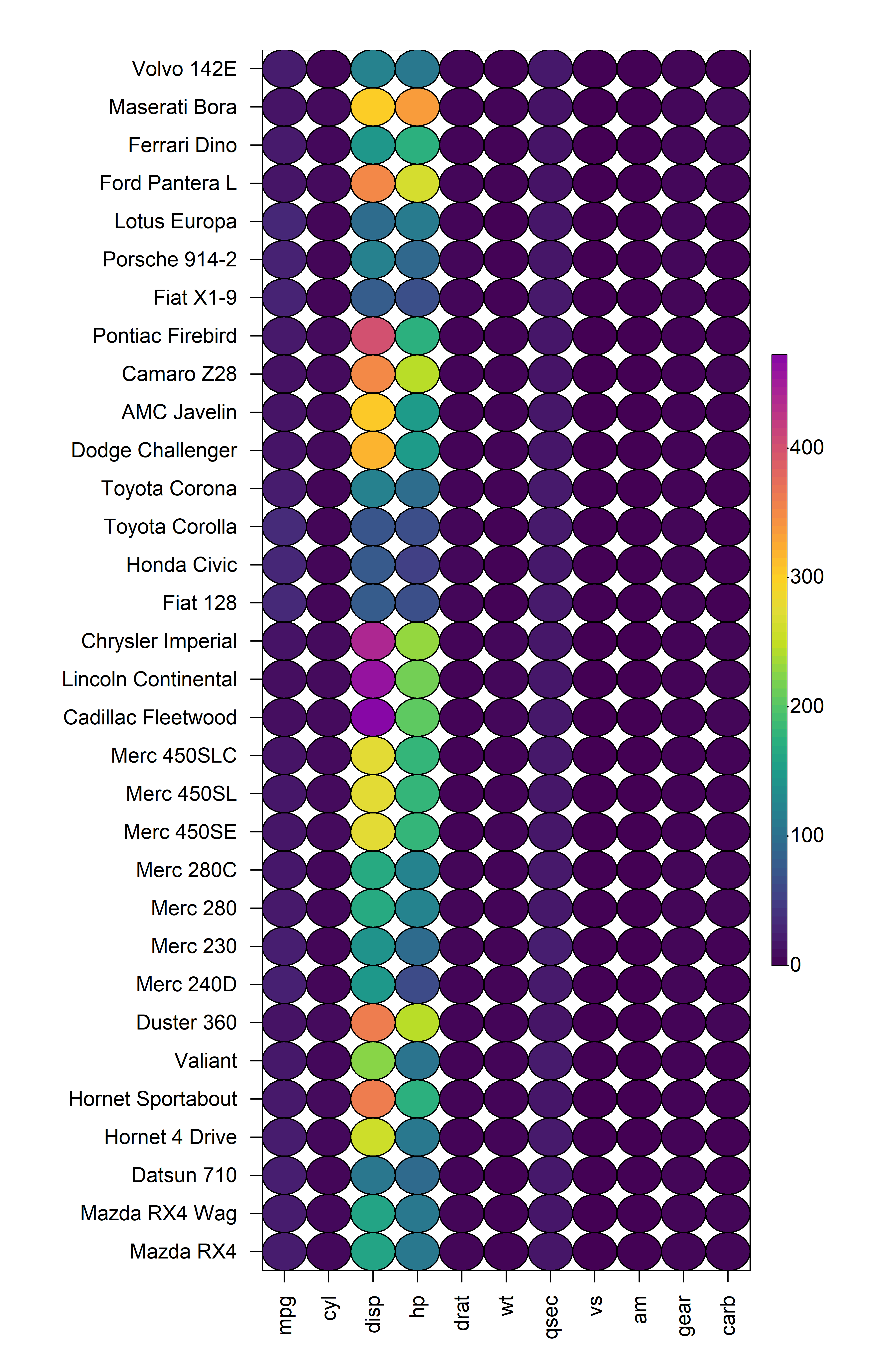
2.1 Cell Shape
heat_map() supports different cell shapes through the
cell_shape argument which can be set to either
"rect" (default), "circle" or
"diamond".
heat_map(
  mtcars,
  cell_shape = "circle"
)
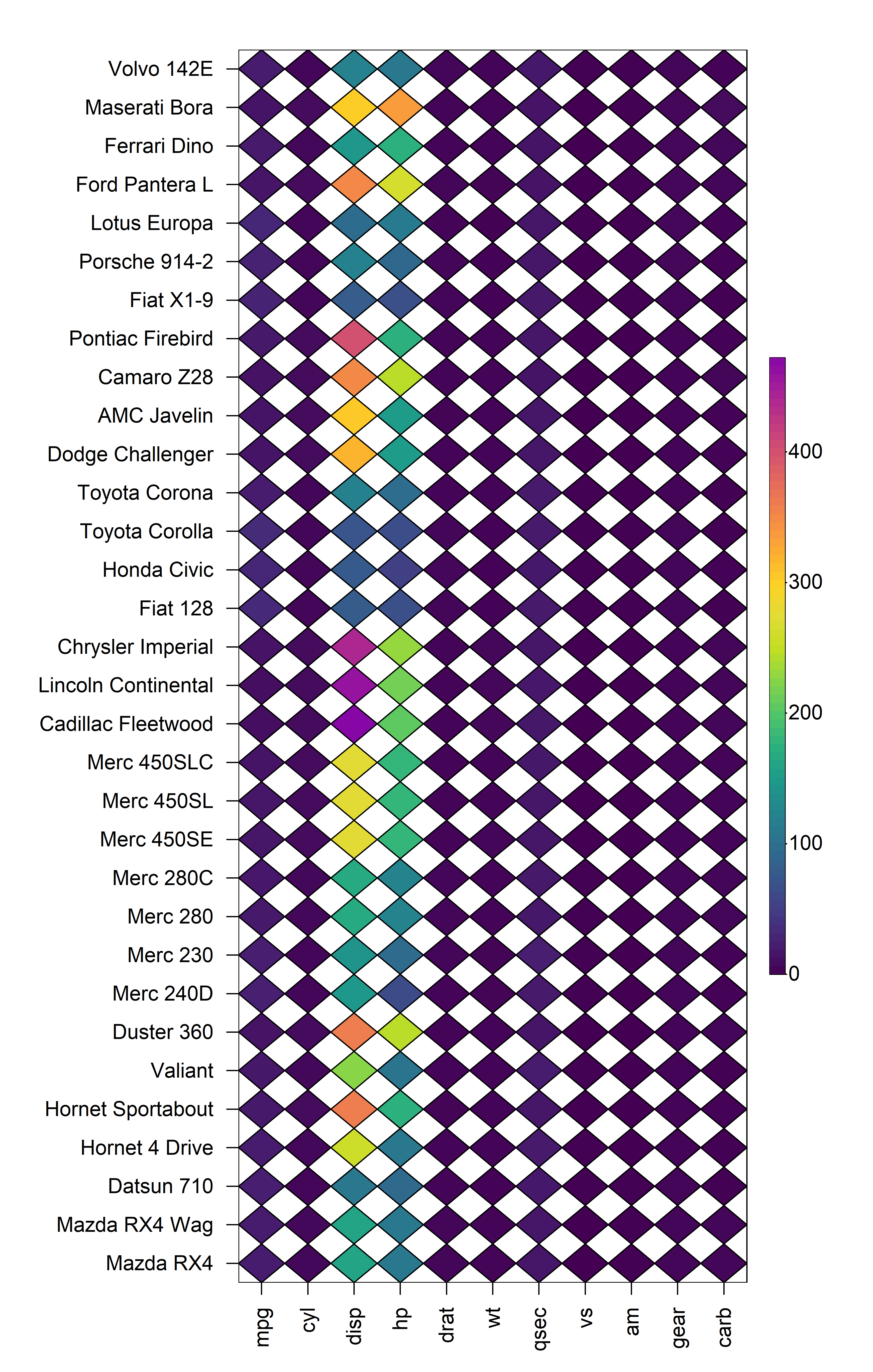
heat_map(
  mtcars,
  cell_shape = "diamond"
)
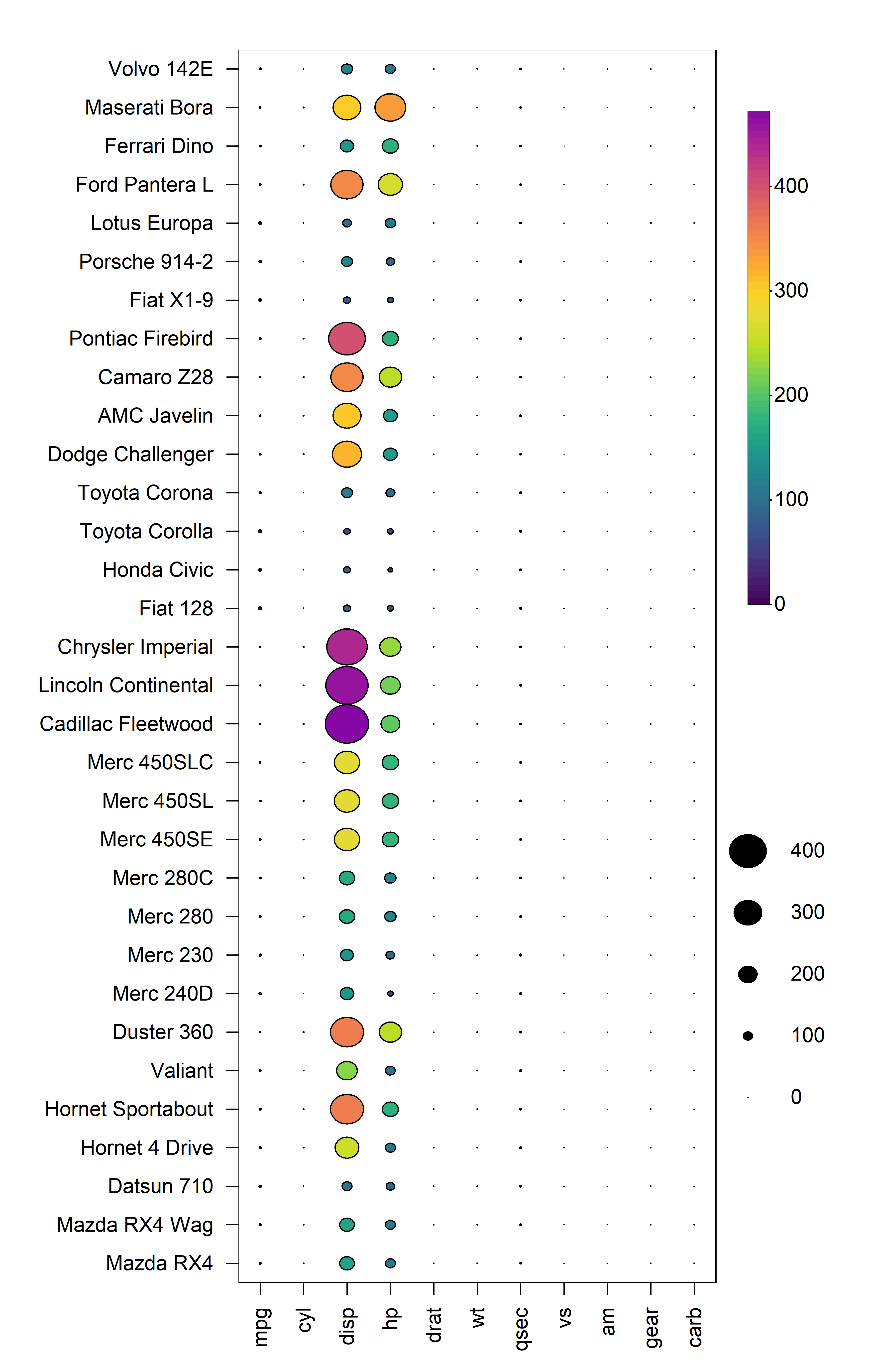
2.2 Cell Size
The size of each cell is controlled through the
cell_size argument. Setting cell_size = TRUE
will scale the size of each cell based on its value in the input matrix.
Alternatively, users can supply a separate matrix of the same
dimensionality and orientation as the input matrix to control the size
of the cells independently of their colour.
heat_map(
  mtcars,
  cell_shape = "circle",
  cell_size = TRUE
)
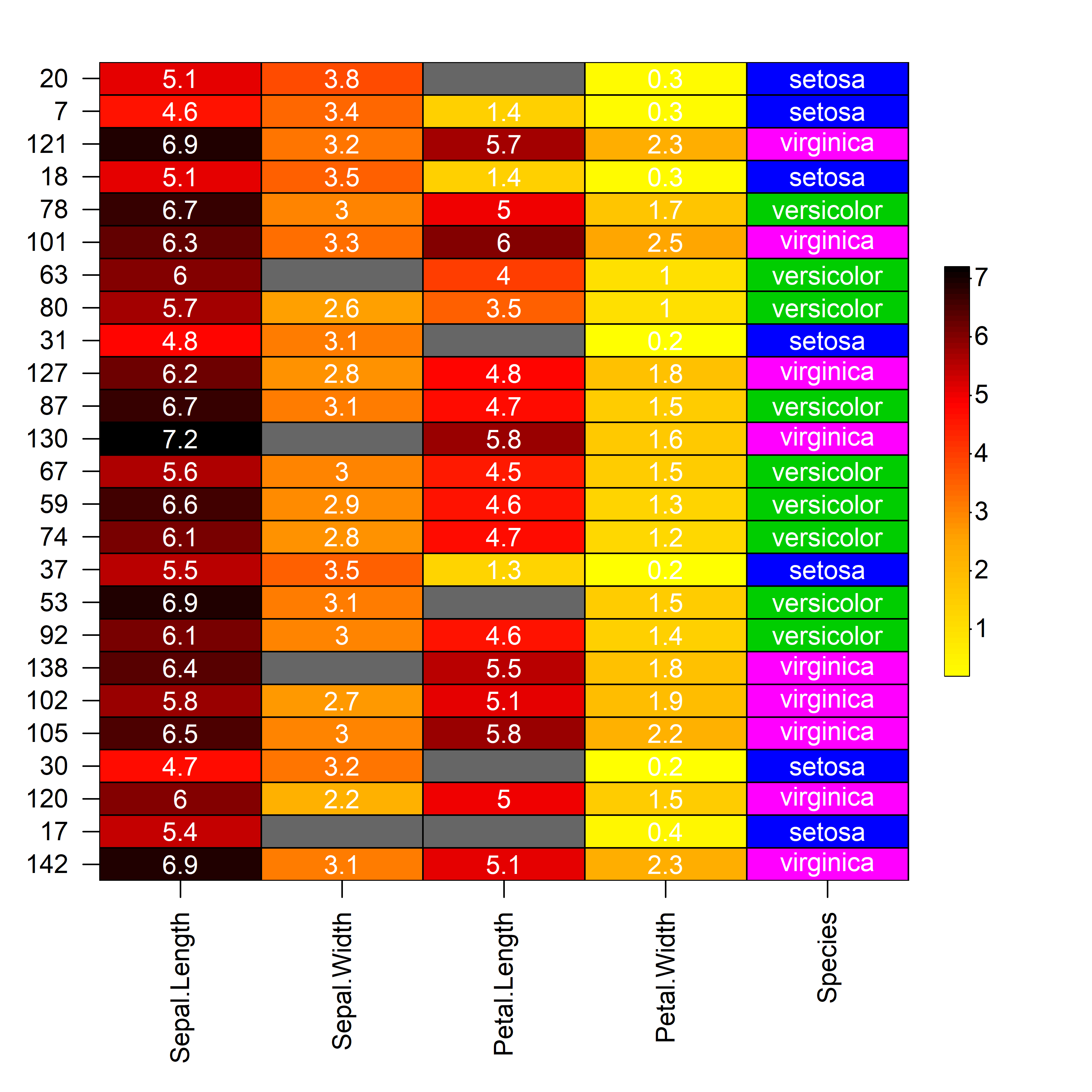
2.3 Cell Colours
The colour of each cell in the heatmap is dependent on the type of
data in that cell. Cells containing numeric values will be assigned
colours based on the continuous colour scale supplied to
cell_col_scale, whilst cells containing non-numeric values
will be assigned colours from the discrete colour palette supplied to
cell_col_palette. Missing values of the form
NA are also supported and the colour of cells containing
missing values can be controlled through the cell_col_empty
argument. The cell_col_alpha argument accepts values
ranging from zero (transparent) to one (solid) to for fine control over
the transparency of the colour in each cell of the heatmap. In the
example below, we will demonstrate the handling of different data types
within heat_map() using a modified subset of the
iris dataset where additional missing values have been
introduced:
# Modified subset of iris dataset with missing values
iris_sub <- iris[sample(1:nrow(iris), 25), ]
iris_sub[c(2, 19, 14, 7), 2] <- NA
iris_sub[c(4, 9, 17, 25), 3] <- NA

# Build heatmap
heat_map(
  iris_sub,
  cell_text = TRUE,
  cell_col_empty = "grey40",
  cell_col_scale = c(
    "yellow",
    "orange",
    "red",
    "black"
  ),
  cell_col_palette = c(
    "magenta",
    "blue",
    "green3"
  ),
  cell_col_alpha = 1
)
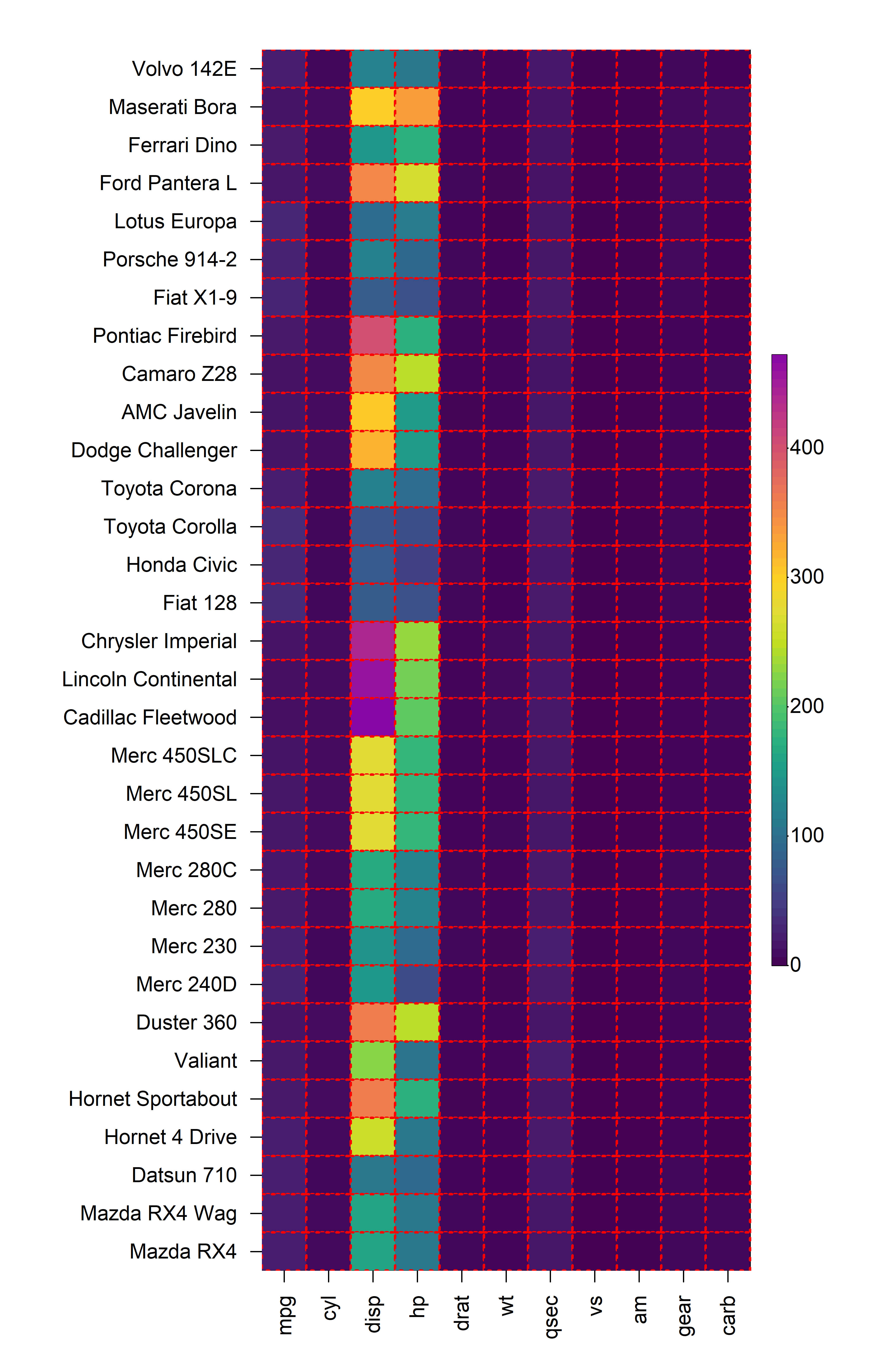
2.4 Cell Borders
The borders of every cell within the constructed heatmap can also be
customised using the cell_border_line_type,
cell_border_line_width, cell_border_line_col
and cell_border_line_col_alpha arguments.
heat_map(
  mtcars,
  cell_border_line_type = 3,
  cell_border_line_width = 2,
  cell_border_line_col = "red",
  cell_border_line_col_alpha = 1
)
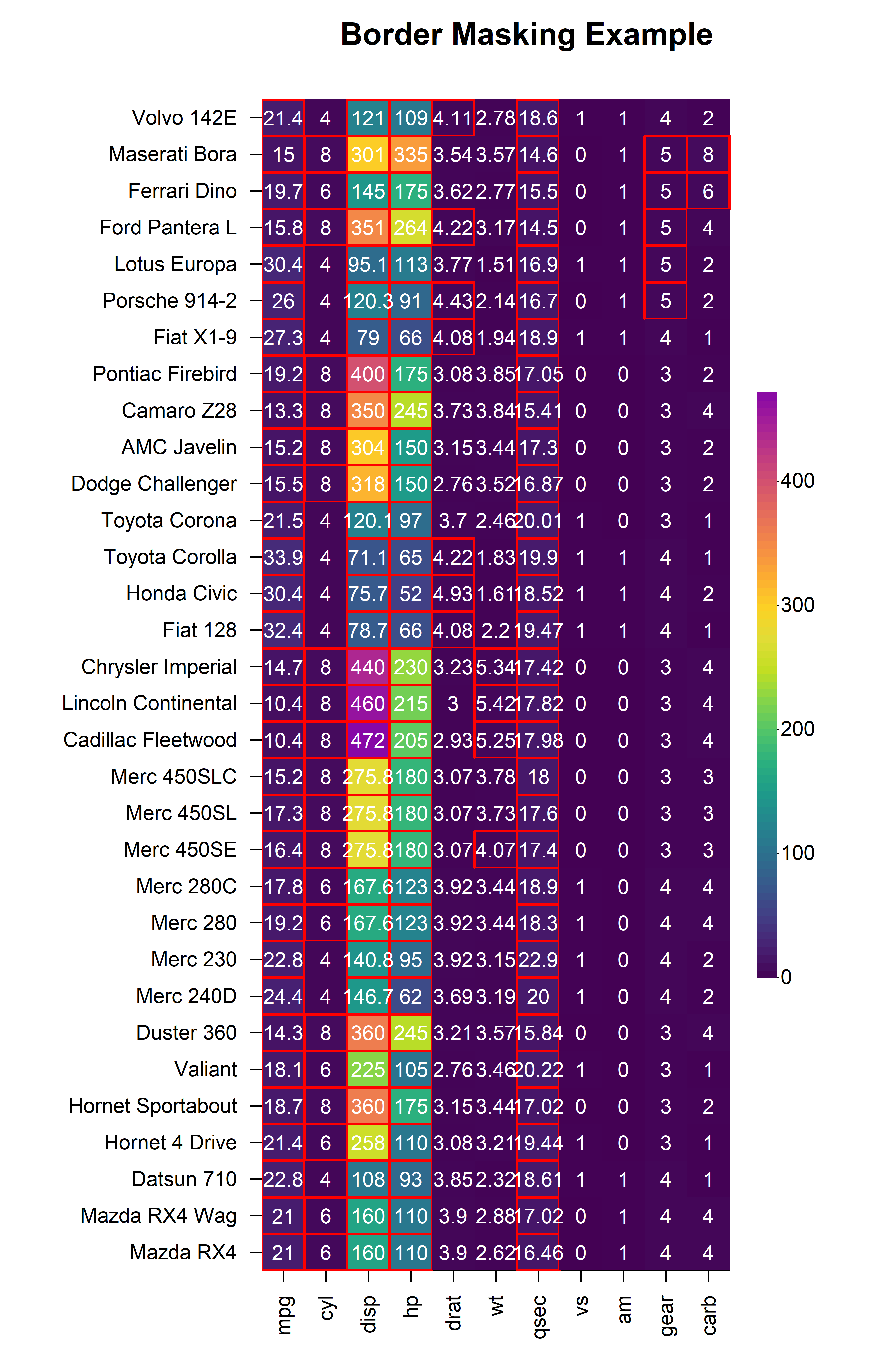
2.4.1 Border Masking
The cell_border_mask argument allows you to selectively
apply colored borders to specific cells by supplying a logical matrix of
the same dimensions as the input data. Cells with TRUE
values will display colored borders, while cells with FALSE
values will have transparent borders. This is particularly useful for
highlighting specific patterns or regions of interest within a
heatmap.
# Create a mask to highlight high values
border_mask <- mtcars > median(unlist(mtcars))

heat_map(
  mtcars,
  cell_border_line_width = 2,
  cell_border_line_col = "red",
  cell_border_mask = border_mask,
  title = "Border Masking Example"
)
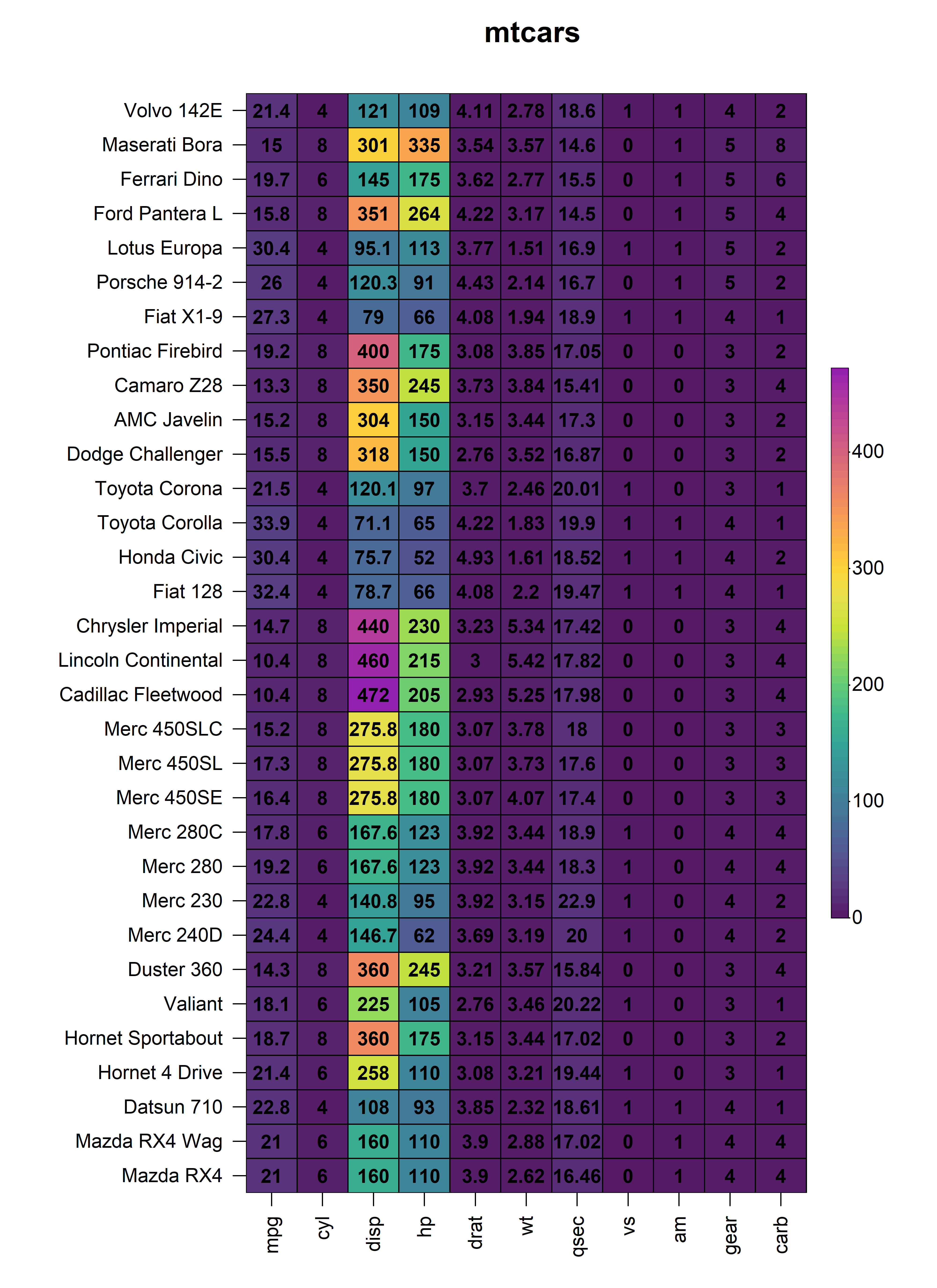
2.5 Cell Text
The values of every cells within the constructed heatmap can be
displayed by setting cell_text = TRUE. By default, numeric
values are rounded to two decimal places but this can be changed through
the round argument. The text displayed in each cell can
easily be customised using the cell_text_size,
cell_text_font, cell_text_col and
cell_text_col_alpha arguments.
heat_map(
  mtcars,
  cell_text = TRUE,
  cell_text_size = 1,
  cell_text_font = 2,
  cell_text_col = "black",
  cell_text_col_alpha = 1,
  title = "mtcars"
)
3. Data Scaling
In the above heatmap, it is very clear that each of the columns of
the input matrix are on completely different scales, making it difficult
to visualise differences in columns with very small values. In order to
represent each column on the same scale, we can apply a form of data
scaling through the scale_method argument either to each
row or column as specified by the scale argument.
Currently, heat_map() has internal support for
"mean", "range" and "z-score"
scaling methods that can be applied to either the rows or columns of the
input matrix.
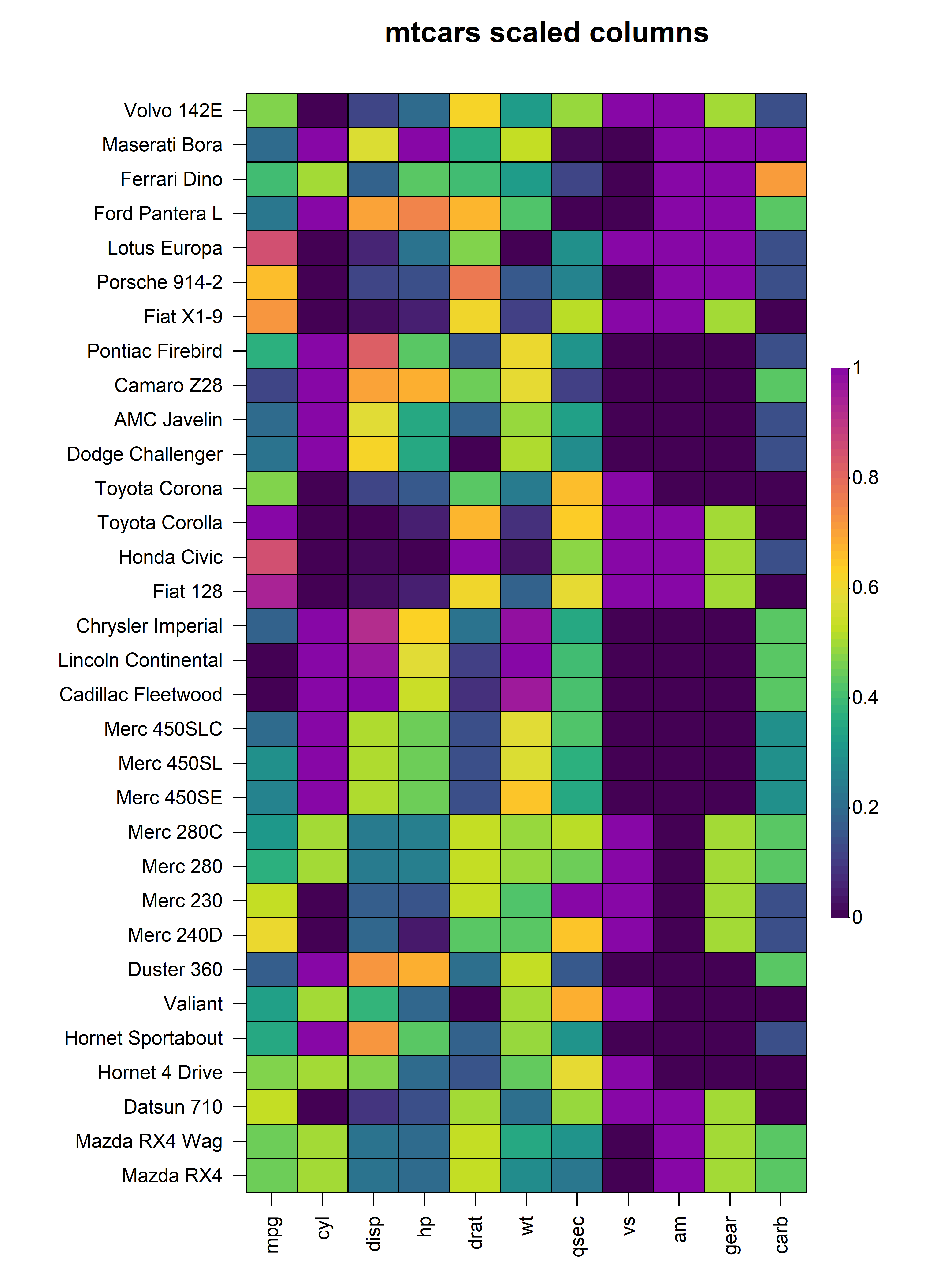
3.1 Scaling Columns
To scale the values in every column, simply set
scale = "column and specify the scaling method through the
scale_method argument. For example, to apply range scaling
to every column in the mtcars dataset:
heat_map(
  mtcars,
  scale = "column",
  scale_method = "range",
  title = "mtcars scaled columns"
)
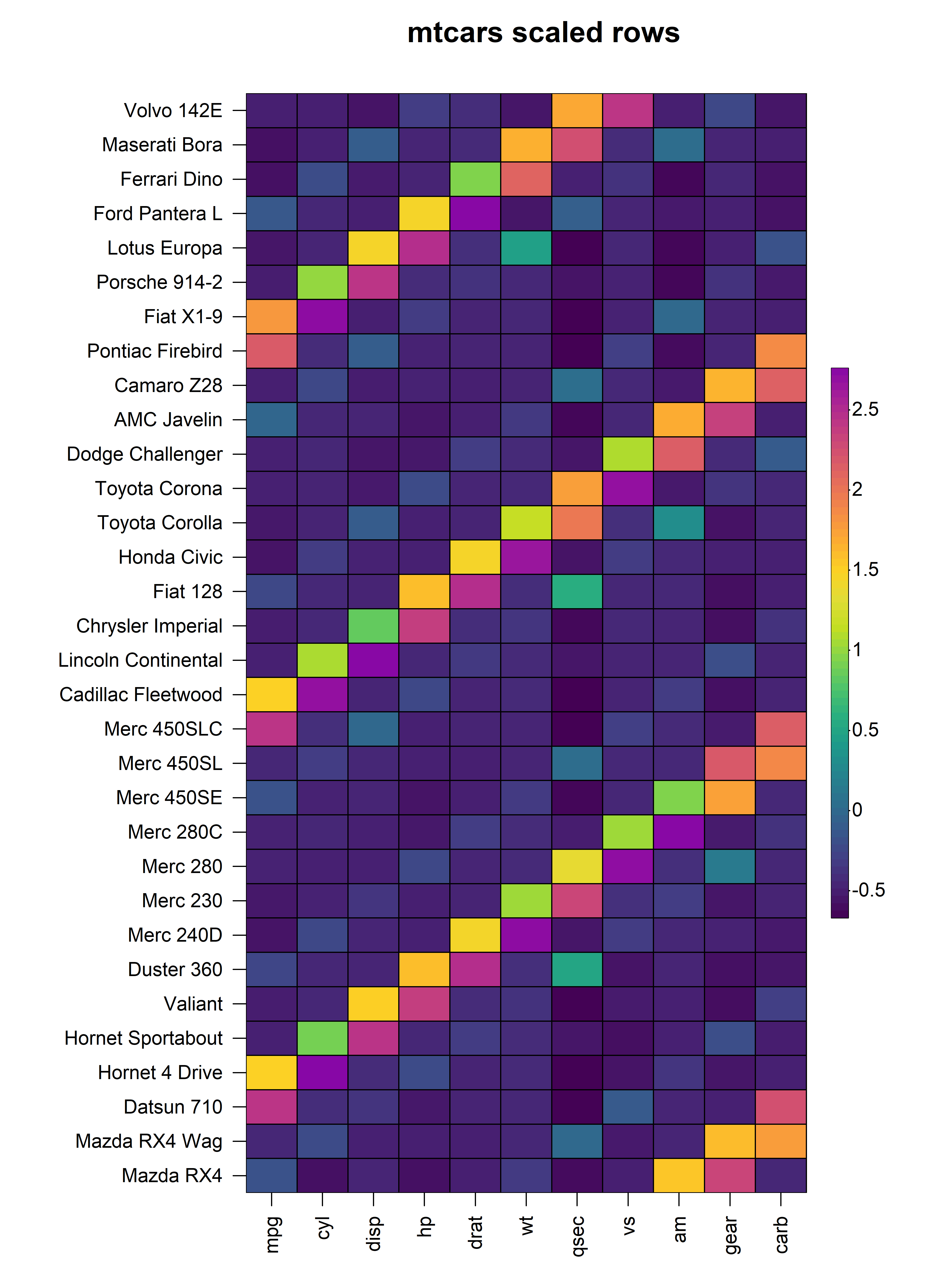
3.2 Scaling Rows
Similarly, in instances where it is more appropriate to scale the
values in each row, we can set scale = "row" and pass the
required scaling method to scale_method. For example, to
apply z-score scaling to every row in the mtcars
dataset:
heat_map(
  mtcars,
  scale = "row",
  scale_method = "zscore",
  title = "mtcars scaled rows"
)
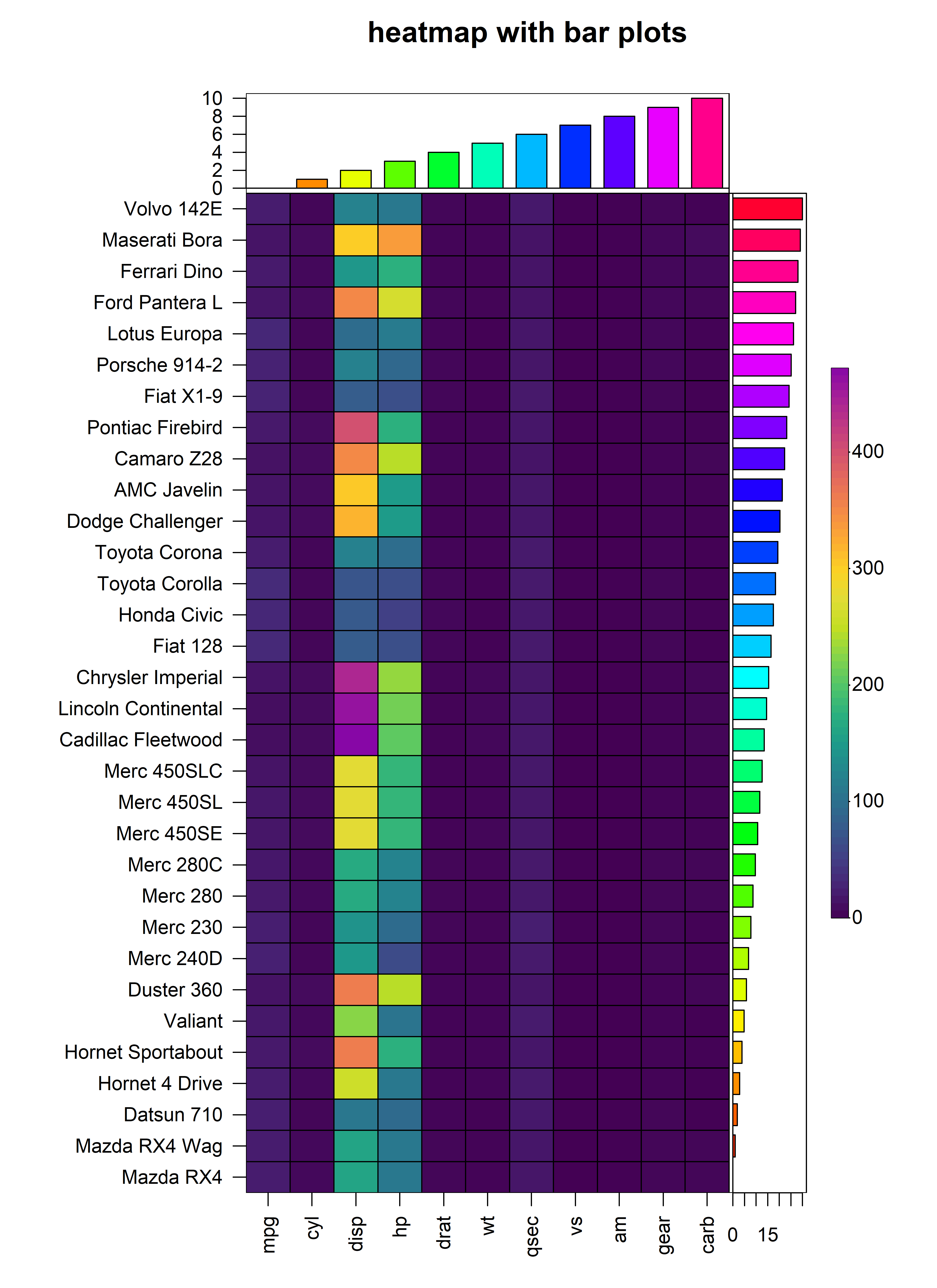
4. Bar Plots
In addition to the cells of the heatmap, heat_map()
supports the display of additional values in bar plots on either axis of
the heatmap. To add bar plots to the heatmap, users should supply the
(named) values to bar_values_x and/or
bar_values_y in the same order as the original input
matrix. The bar plots will be displayed on the opposite side to the axis
text and size of the bar plot (i.e. height or width) can be controlled
through the bar_size_x and bar_size_y
arguments. The colours of the bars and borders can be customised using
the bar_fill_ and bar_line_ family of
arguments. In the example below, we demonstrate the addition of bar
plots to the x and y axes of a heatmap constructed using the
mtcars dataset:
heat_map(
  mtcars,
  bar_values_x = 1:ncol(mtcars),
  bar_size_x = 0.5,
  bar_fill_x = rainbow(ncol(mtcars)),
  bar_line_col_x = "black",
  bar_values_y = 1:nrow(mtcars),
  bar_size_y = 0.8,
  bar_fill_y = rainbow(ncol(mtcars)),
  bar_line_col_y = "black",
  title = "heatmap with bar plots"
)
5. Hierarchical Clustering
heat_map() also supports hierarchical clustering using
the conventional stats::hclust() to construct dendrograms
and stats::cutree() to partition the dendrograms into
distinct clusters. The dist_method and
clust_method arguments allow for control over the distance
metric to use for hierarchical clustering (any method supported by
stats::dist() or "cosine" for cosine distance)
and the agglomeration method to use (any method supported by
stats::hclust()).
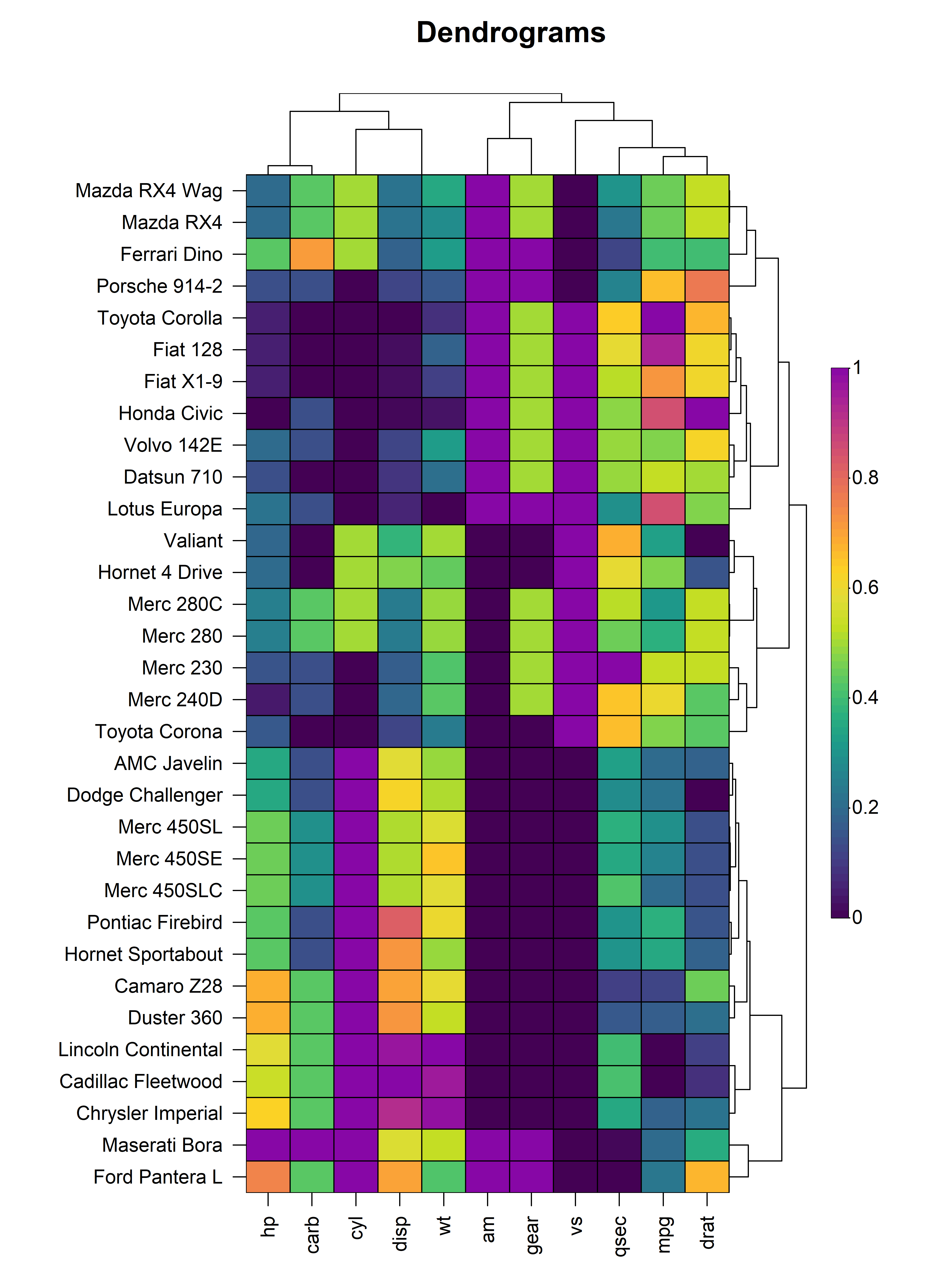
5.1 Dendrograms
Dendrograms can be added to the x and/or y axis using the
tree, tree_x or tree_y arguments.
The tree argument indicates whether dendrograms should be
drawn for the "x", "y" or "both"
axes. Alternatively, the tree_x or tree_y
arguments can be set to TRUE to include dendrograms on the
x or y axes respectively. The tree_x and
tree_y arguments also accept objects of class
dist or hclust to allow for custom dendrograms
using unsupported distance metrics or agglomeration methods. The
tree_size_x and tree_size_y arguments are
scalars to control the height or width of the dendrograms on the x and y
axes respectively. The tree_scale_x and
tree_scale_y arguments can be used to scale the branch
heights of the dendrogram to be the same height at each level allowing
for better visualisation of relationships in large heatmaps.
heat_map(
  mtcars,
  scale = "column",
  dist_method = "euclidean",
  clust_method = "complete",
  tree_x = TRUE,
  tree_size_x = 0.4,
  tree_y = TRUE,
  tree_size_y = 0.8,
  title = "Dendrograms"
)
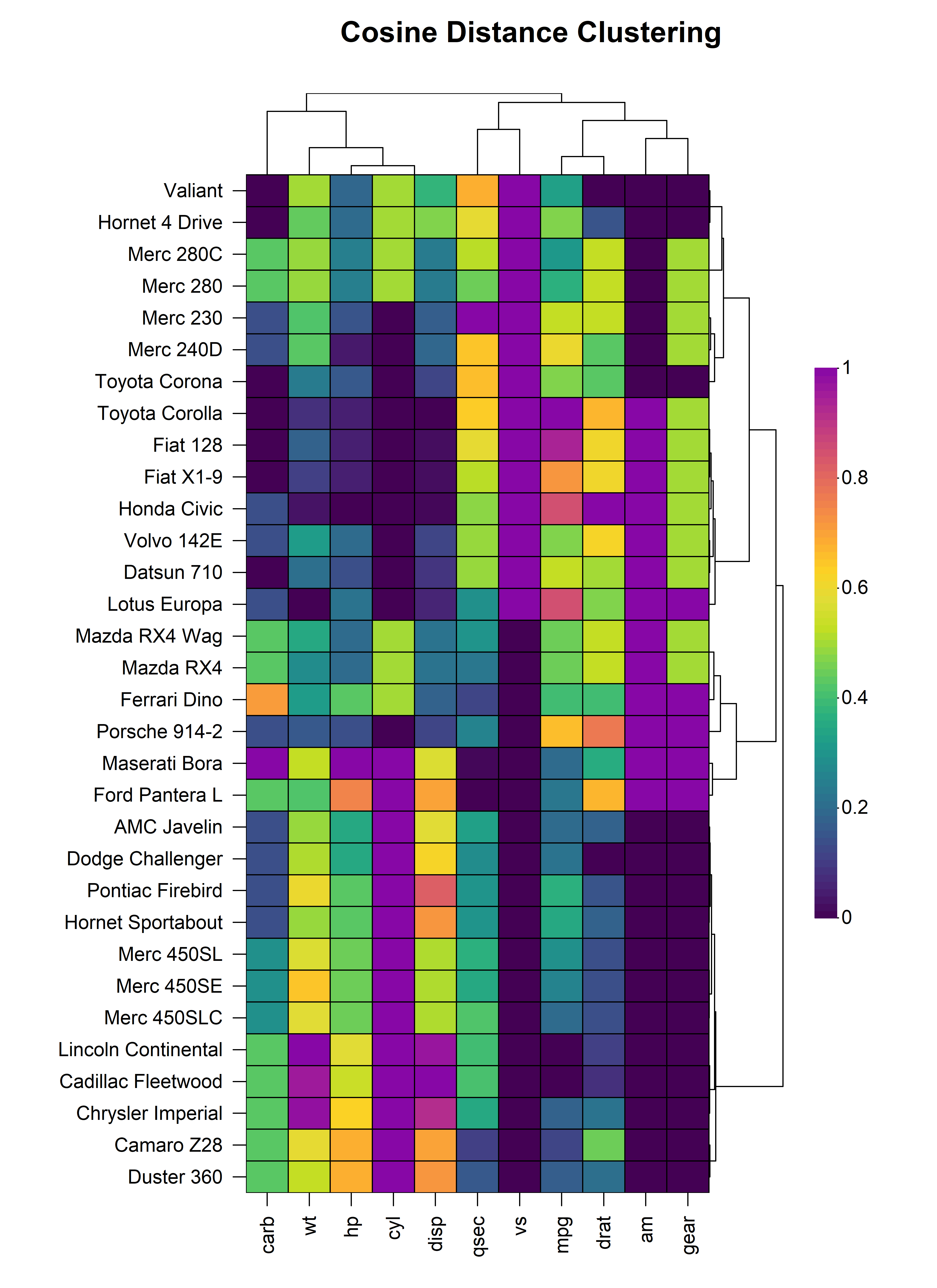
5.1.1 Cosine Distance
In addition to the standard distance metrics supported by
stats::dist(), HeatmapR also supports
cosine distance for hierarchical clustering. Cosine distance (1 - cosine
similarity) measures the angle between vectors and is particularly
useful for high-dimensional data where the magnitude of the vectors is
less important than their direction. This is especially valuable when
analyzing gene expression data or other normalized datasets.
heat_map(
  mtcars,
  scale = "column",
  dist_method = "cosine",
  clust_method = "complete",
  tree_x = TRUE,
  tree_size_x = 0.4,
  tree_y = TRUE,
  tree_size_y = 0.8,
  title = "Cosine Distance Clustering"
)
Absolute Distance Thresholds: When using cosine
distance, tree_cut values between 0 and 1 are interpreted
as absolute cosine distance thresholds rather than proportional tree
heights. For example, tree_cut_x = 0.5 means cluster at
cosine distance of 0.5, not at 50% of the tree height. This provides
more intuitive control over clustering based on actual distance
values.
# Cut at absolute cosine distance of 0.5
heat_map(
mtcars,
scale = "column",
dist_method = "cosine",
tree_x = TRUE,
tree_cut_x = 0.5,
tree_split_x = 1,
title = "Cosine Distance with Absolute Threshold"
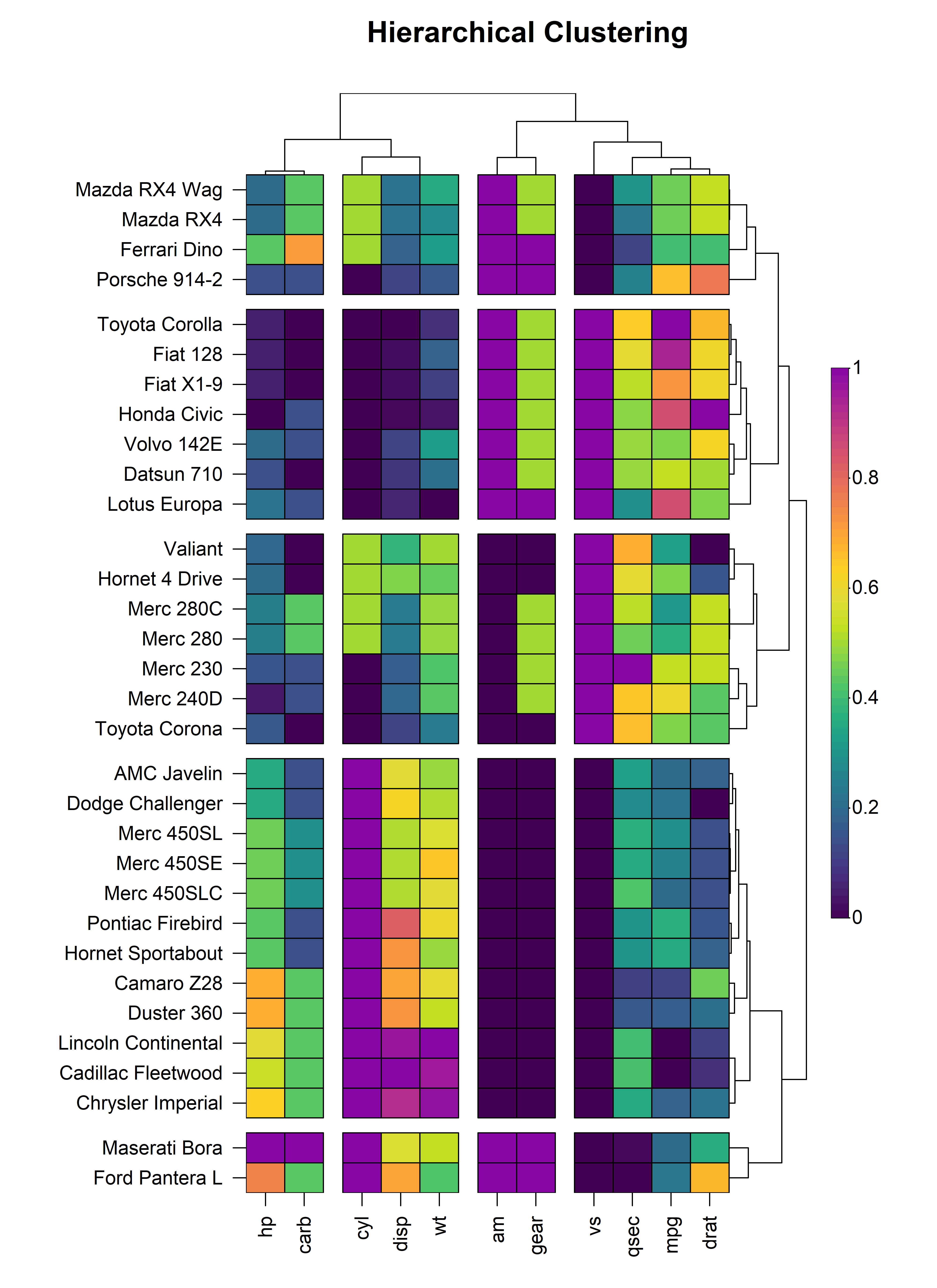
)5.2 Clustering
The dendrograms on either axis can be optionally cut to reveal
clusters in the data. Dendrogram cutting is performed via the
tree_cut_x and tree_cut_y arguments which
accept either a fixed number of clusters or a proportion of the total
dendrogram height where the cut should be made. The clusters can be
spatially separated by introducing splits in the heatmap using the
tree_split_x and tree_split_y arguments which
are scalars that control the height or width of the splits.
heat_map(
  mtcars,
  scale = "column",
  dist_method = "euclidean",
  clust_method = "complete",
  tree_x = TRUE,
  tree_size_x = 0.4,
  tree_cut_x = 4,
  tree_split_x = 1,
  tree_y = TRUE,
  tree_size_y = 0.8,
  tree_cut_y = 5,
  tree_split_y = 1,
  title = "Hierarchical Clustering"
)
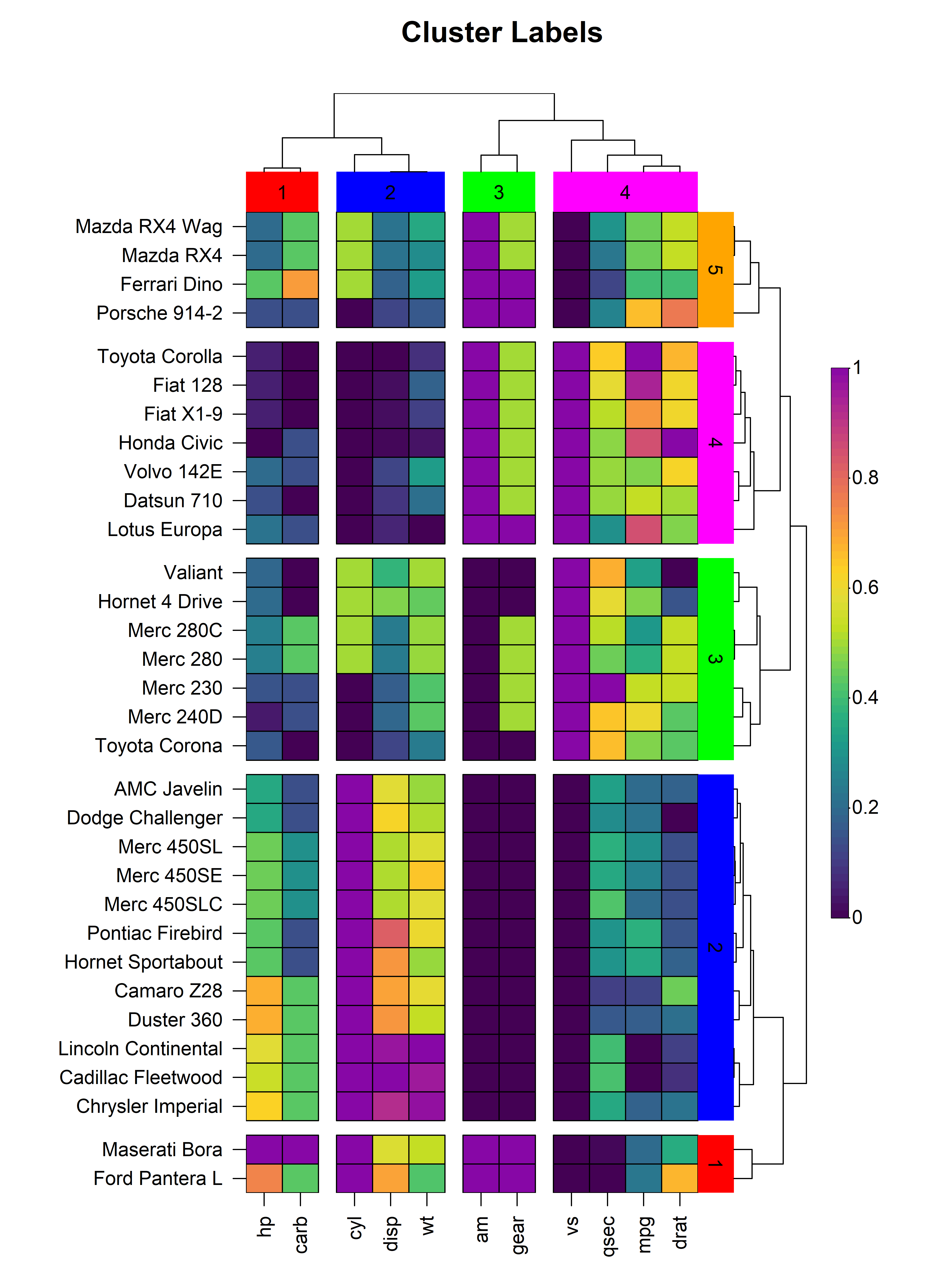
In addition to heatmap splitting, heat_map() also
supports the labelling of clusters through the
tree_label_x, tree_label_text_x,
tree_label_y and tree_label_text_y
arguments.
heat_map(
  mtcars,
  scale = "column",
  tree_size_x = 0.4,
  tree_cut_x = 4,
  tree_split_x = 1,
  tree_label_x = TRUE,
  tree_label_size_x = 1.4,
  tree_label_text_x = c(1:4),
  tree_label_col_x = c(
    "red",
    "blue",
    "green",
    "magenta"
  ),
  tree_y = TRUE,
  tree_size_y = 0.8,
  tree_cut_y = 5,
  tree_split_y = 1,
  tree_label_y = TRUE,
  tree_label_size_y = 1,
  tree_label_text_y = c(1:5),
  tree_label_col_y = c(
    "red",
    "blue",
    "green",
    "magenta",
    "orange"
  ),
  title = "Cluster Labels"
)
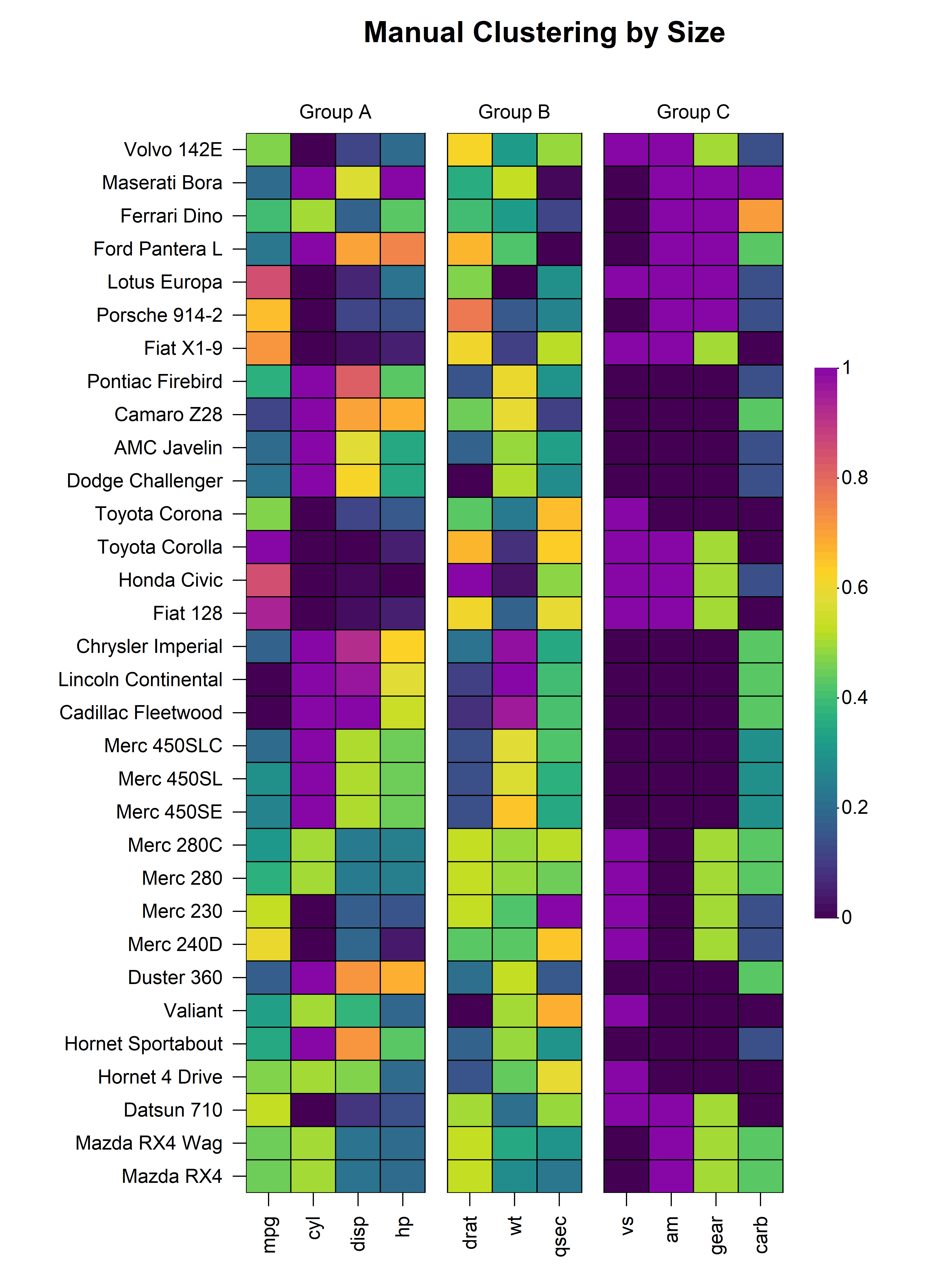
5.2.1 Manual Clustering
In addition to automatic hierarchical clustering, HeatmapR allows you to manually define clusters in two ways: by specifying the number of elements in each cluster, or by providing a vector of cluster indices. This is particularly useful when you want to group data based on domain knowledge or external factors rather than hierarchical relationships.
Method 1: Specify cluster sizes - Provide a vector indicating the number of rows/columns in each cluster:
# Manual clustering by specifying cluster sizes
# Create 3 clusters: 4 columns, 3 columns, 4 columns
heat_map(
  mtcars,
  scale = "column",
  tree_cut_x = c(4, 3, 4),
  tree_split_x = 1,
  tree_label_x = TRUE,
  tree_label_text_x = c("Group A", "Group B", "Group C"),
  title = "Manual Clustering by Size"
)
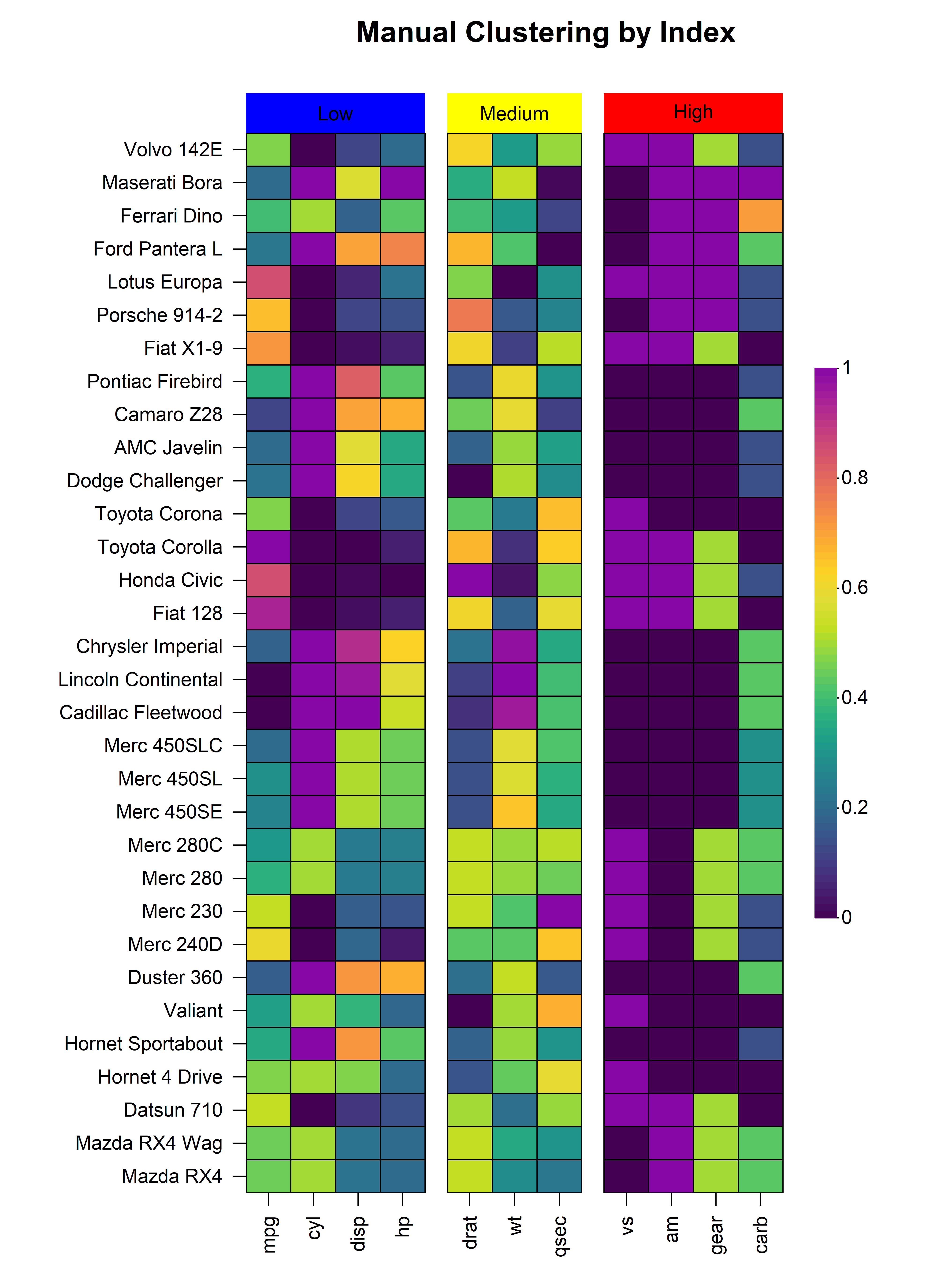
Method 2: Specify cluster indices - Provide a vector where each element indicates which cluster that row/column belongs to:
# Manual clustering by assigning cluster indices
# Assign each of the 11 columns to specific clusters
cluster_indices <- c(1, 1, 1, 1, 2, 2, 2, 3, 3, 3, 3)

heat_map(
  mtcars,
  scale = "column",
  tree_cut_x = cluster_indices,
  tree_split_x = 1,
  tree_label_x = TRUE,
  tree_label_text_x = c("Low", "Medium", "High"),
  tree_label_col_x = c("blue", "yellow", "red"),
  title = "Manual Clustering by Index"
)
Manual clustering can be combined with dendrograms by setting
tree_x = TRUE or tree_y = TRUE, allowing you
to display the hierarchical relationships while still using your custom
cluster definitions.
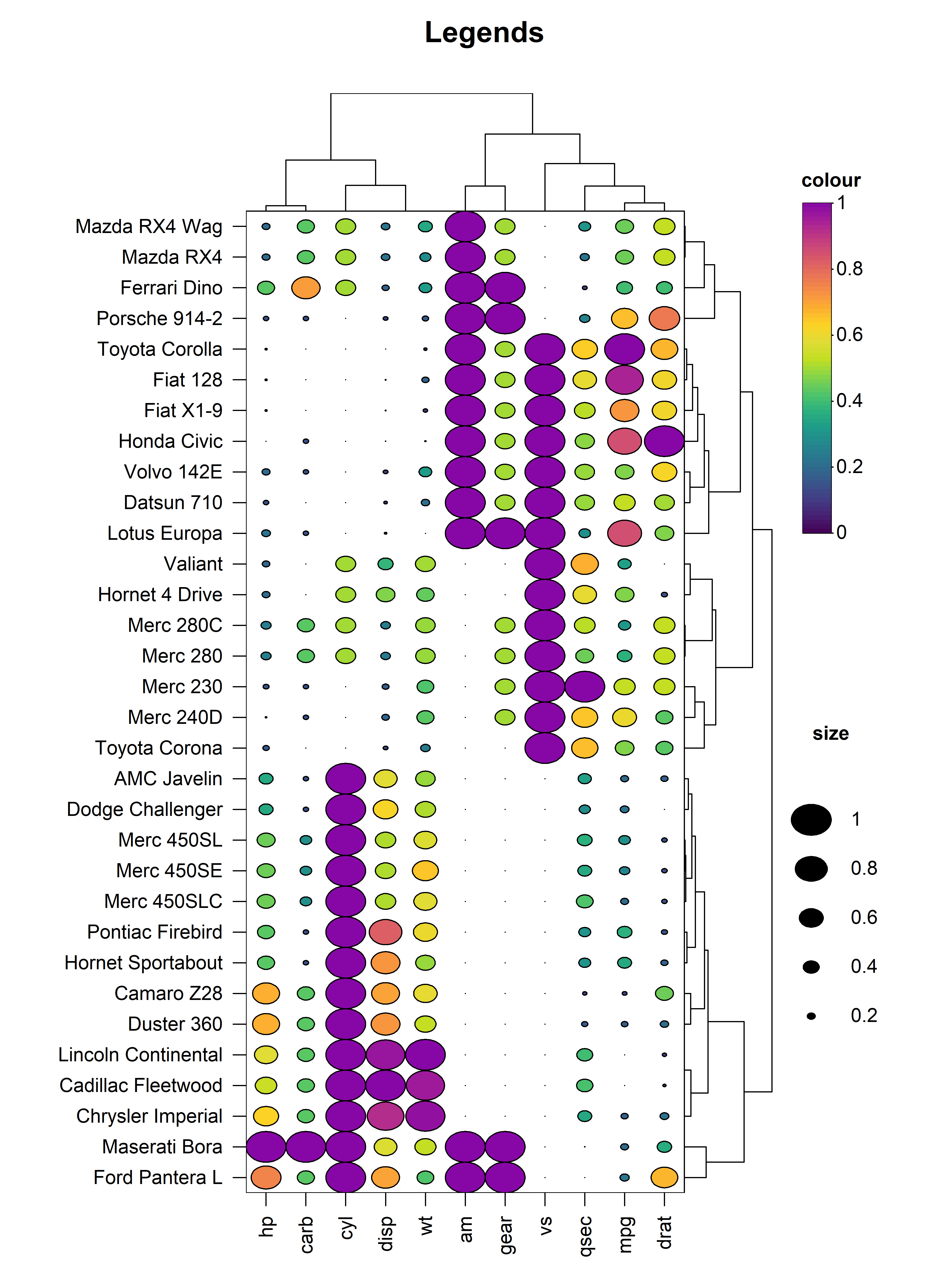
6. Legends
heat_map() will automatically add legends for the colour
scale and size of the cells in the heatmap. The legend
argument controls the type(s) of legends to display including the
"colour", "shape" or "both". The
space available to the legend can be tweaked using the
legend_size argument, and the size of the colour scale
legend can be controlled through the legend_col_scale_size
argument. The titles and text displayed in the legend(s) are also fully
customisable using the the legend_title_ and
legend_text_ family of arguments.
heat_map(
  mtcars,
  scale = TRUE,
  tree_x = TRUE,
  tree_y = TRUE,
  cell_shape = "circle",
  cell_size = TRUE,
  legend = TRUE,
  legend_size = 1.5,
  legend_col_scale_size = 1.2,
  legend_title = c("colour", "size"),
  title = "Legends"
)
7. Complex Layouts
HeatmapR supports the arrangement of multiple heatmaps
in complex layouts using heat_map_custom().
heat_map_custom() is called prior to plotting to open the
appropriate graphics device and set the desired layout before adding the
heatmaps. Once the layout is complete, a call is made to
heat_map_complete() to reset all heat_map()
associated settings. The layout argument can be either a
vector indicating the desired number of rows and columns or a mtrix
defining a more complex layout. For example, if we want to split
different car brands into separate heatmaps and arrange them:
heat_map_custom(
  popup = TRUE,
  popup_size = c(10, 15),
  layout = matrix(
    c(1,1,2,2,1,1,3,3),
    ncol = 4,
    nrow = 2,
    byrow = TRUE
  )
)
heat_map(
  mtcars[grepl("Merc", rownames(mtcars)),],
  title = "Mercedes"
)
heat_map(
  mtcars[grepl("Mazda|Toyota", rownames(mtcars)),],
  title = "Mazda | Toyota"
)
heat_map(
  mtcars[grepl("Hornet|Datsun|Volvo", rownames(mtcars)),],
  title = "Hornet | Datsun | Volvo"
)
heat_map_complete()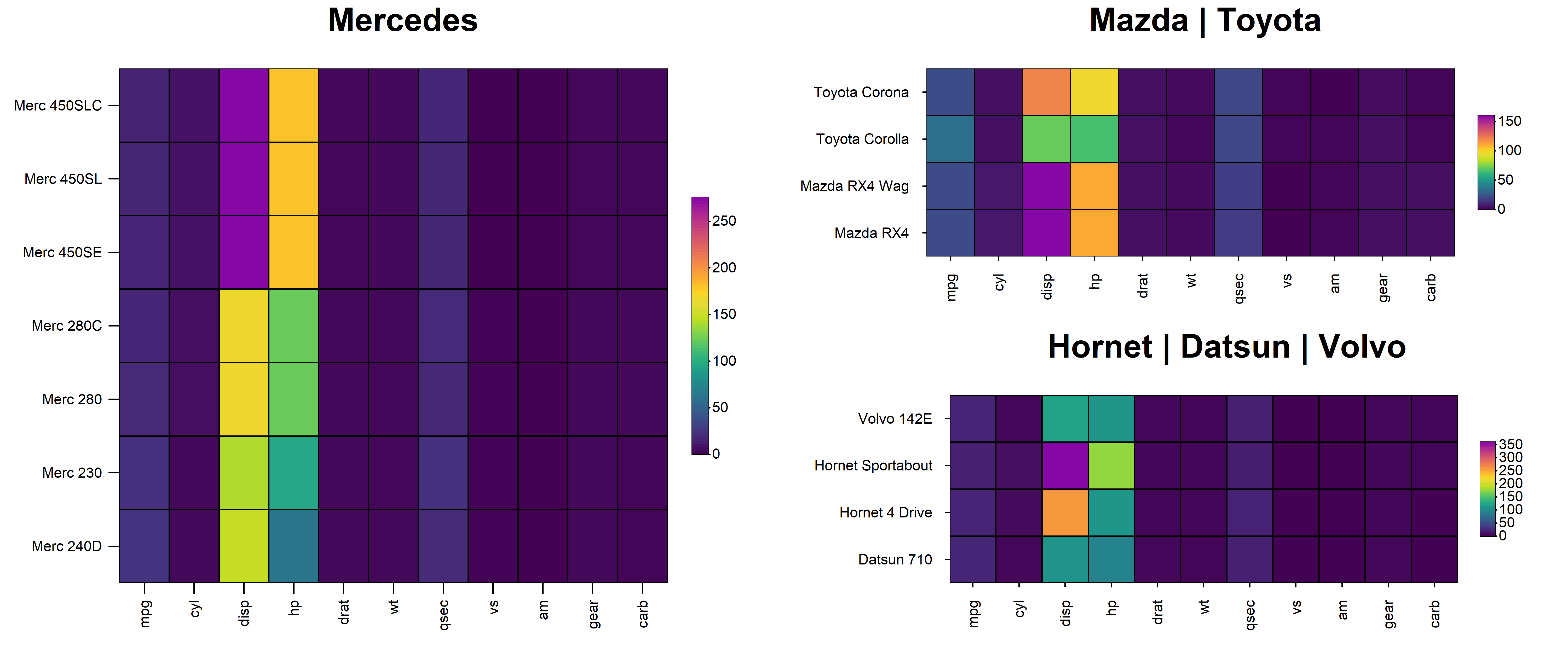
HeatmapR also supports layouts with other plots
generated using base graphics. For example, we could arrange a heatmap
with a scatterplot and a boxplot.
heat_map_custom(
  popup = TRUE,
  popup_size = c(10, 15),
  layout = matrix(
    c(1,1,2,2,1,1,3,3),
    ncol = 4,
    nrow = 2,
    byrow = TRUE
  )
)
heat_map(
  mtcars,
  title = "mtcars"
)
plot(
  mtcars[, c("disp", "hp")],
  xlab = "Displacement",
  ylab = "Horsepower",
  main = "mtcars: Displacement vs Horsepower",
  pch = 16,
  col = "black"
)
boxplot(
  mtcars[, "disp"],
  main = "Displacement",
  xlab = "Displacement (cu.in.)",
  horizontal = TRUE
)
heat_map_complete()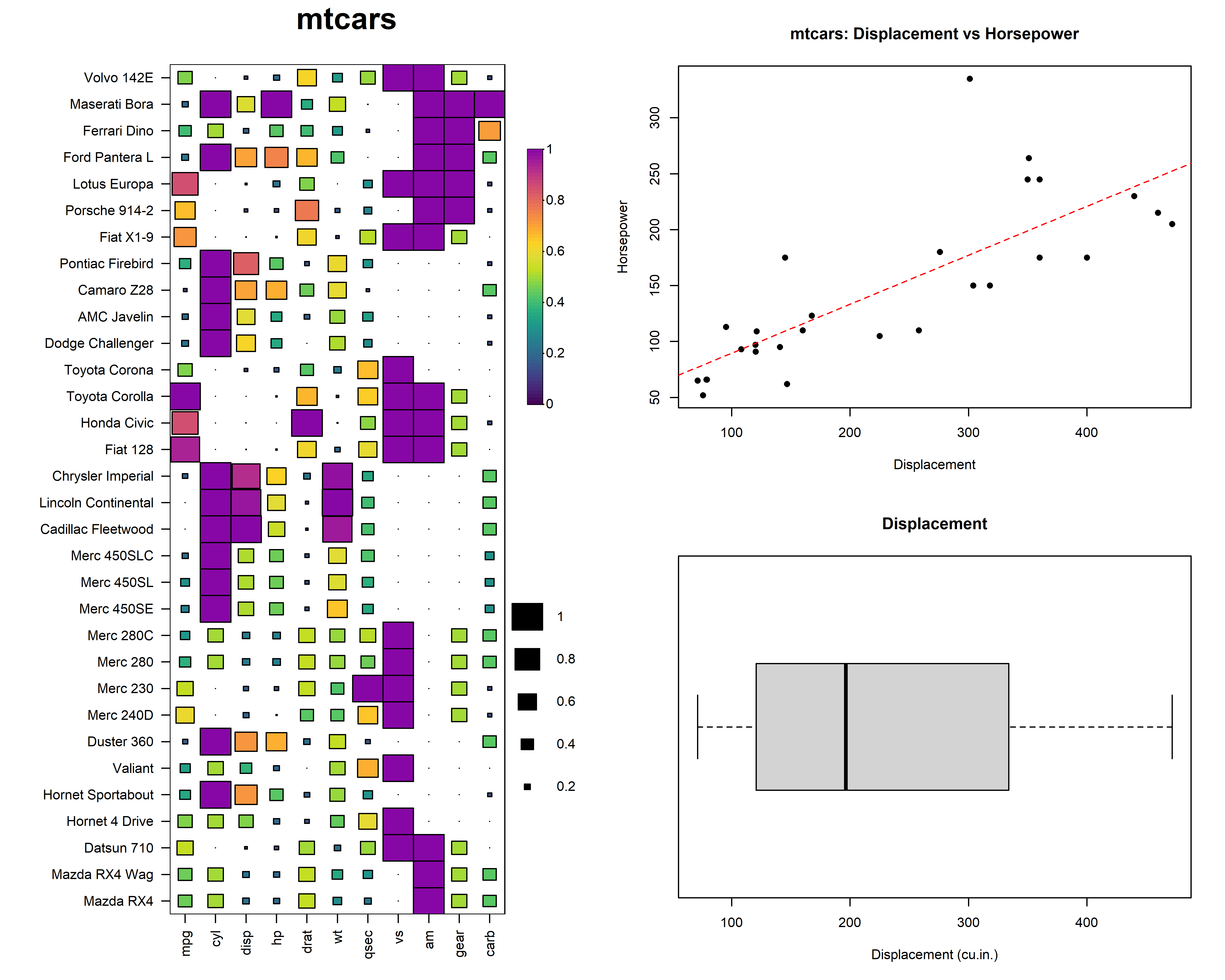
8. Export
HeatmapR supports the export of high resolution images
using heat_map_save() which allows control over the
dimensions and resolution of the exported image.
heat_map_save(
"mtcars.png",
height = 9.5,
width = 5.7,
res = 500
)
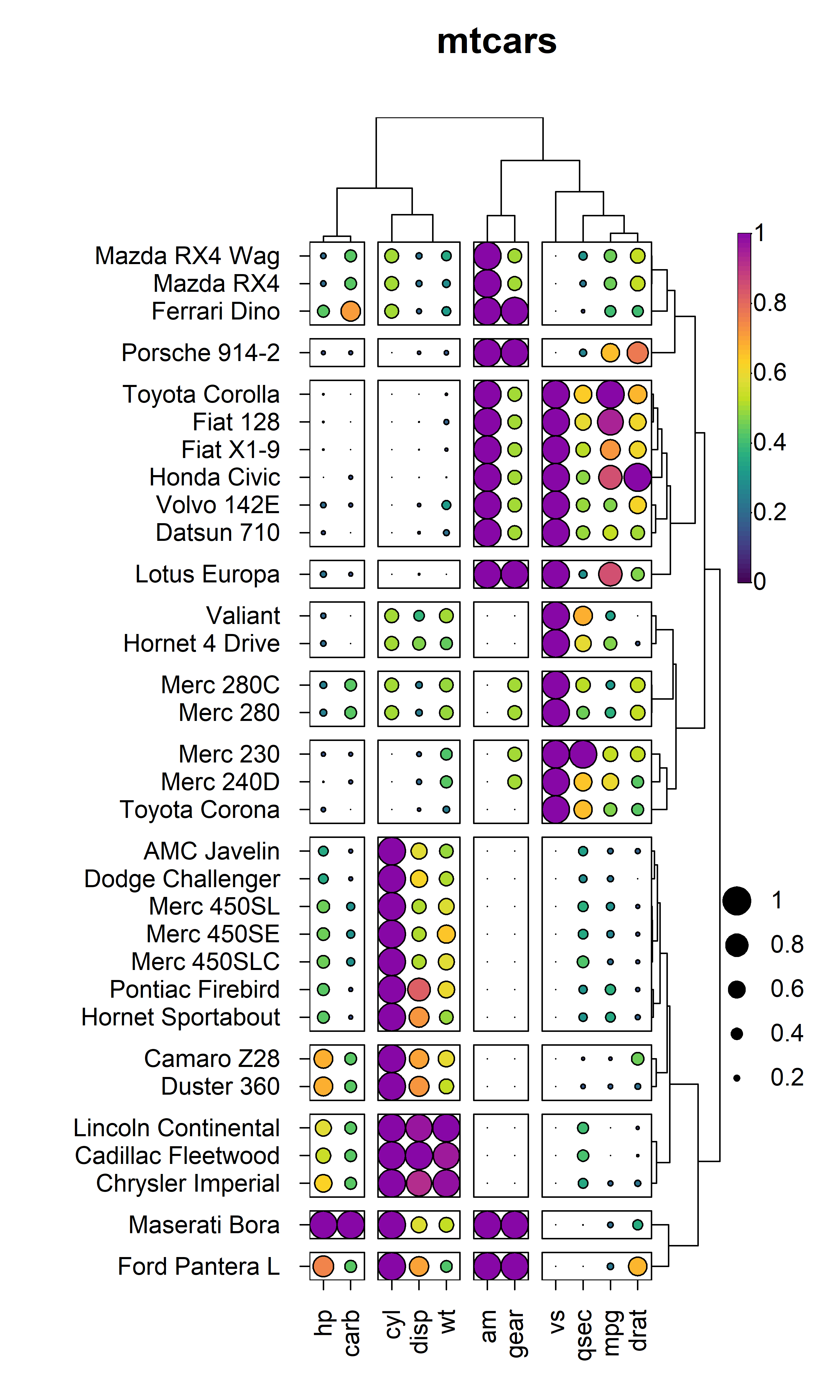
heat_map(
mtcars,
scale = "column",
scale_method = "range",
tree_x = TRUE,
tree_y = TRUE,
tree_cut_x = 4,
tree_cut_y = 12,
cell_size = TRUE,
cell_shape = "circle",
title = "mtcars"
)
heat_map_complete()